كيف تجمع القيم بين تاريخين في Excel؟
عندما تكون لديك قائمتان في ورقة العمل، كما في لقطة الشاشة أدناه—إحداهما تواريخ والأخرى قيم—وترغب في جمع القيم التي تقع ضمن نطاق تاريخي معيّن (مثل جمع القيم بين 3/4/2014 و5/10/2014)، فكيف يمكنك حساب ذلك بسرعة؟ سأعرض لك الآن صيغة فعّالة لجمع هذه القيم في Excel.
جمع القيم بين تاريخين باستخدام صيغة في Excel
لحسن الحظ، توجد صيغة في Excel قادرة على جمع القيم بين تاريخين.
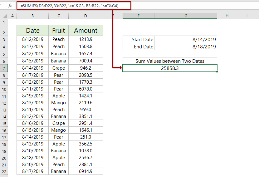
حدد خلية فارغة، وأدخل الصيغة أدناه، ثم اضغط على زرEnter — وستحصل فورًا على نتيجة الحساب. انظر لقطة الشاشة:
=SUMIFS(B2:B8,A2:A8,">="&E2,A2:A8,"<="&E3)
ملاحظة: في الصيغة أعلاه،
- D3:D22هي قائمة القيم التي ستقوم بجمعها
- B3:B22هي قائمة التواريخ التي ستعتمد عليها في الجمع
- G3هي الخلية التي تحتوي على تاريخ البدء
- G4هي الخلية التي تحتوي على تاريخ الانتهاء
 | هل الصيغة معقدة للغاية بحيث يصعب تذكّرها؟ احفظ الصيغة كإدخال نص تلقائي لإعادة استخدامها بنقرة واحدة فقط في المستقبل! قراءة المزيد… تجربة مجانية |
اجمع البيانات بسهولة كل السنة المالية، أو كل نصف السنة، أو كل أسبوع في Excel
تتيح لك ميزة «تجميع الوقت الخاص» في الجداول المحورية من Kutools لـ Excel إضافة عمود مساعد لحساب السنة المالية أو نصف السنة أو رقم الأسبوع أو يوم الأسبوع بناءً على عمود تاريخ معيّن، مما يمكّنك بسهولة من العد أو الجمع أو حساب المتوسط للبيانات وفقًا للنتائج المحسوبة في جدول محوري جديد.
Kutools لـ Excel- عزِّز Excel بقوة أكثر من 300 أداة أساسية، لتجعل عملك أسرع وأسهل، واستفد من ميزات الذكاء الاصطناعي لمعالجة البيانات بشكل أكثر ذكاءً وزيادة الإنتاجية.احصل عليه الآن
جمع القيم بين تاريخين باستخدام التصفية في Excel
إذا كنت بحاجة إلى جمع القيم بين تاريخين، وكان نطاق التاريخ يتغيّر باستمرار، يمكنك تطبيق إضافة المجموعة على النطاق المحدد، ثم استخدام دالة SUBTOTAL لجمع القيم ضمن النطاق التاريخي المطلوب في Excel.
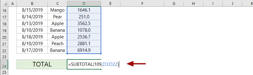
1. حدد خلية فارغة، وأدخل الصيغة أدناه، ثم اضغط مفتاح Enter.
=SUBTOTAL(109,D3:D22)
ملاحظة: في الصيغة أعلاه، يشير 109 إلى جمع القيم المُرشَّحة، بينما يشير D3:D22 إلى نطاق القيم التي سيتم جمعها.
2. حدد عنوان النطاق، ثم انقر علىبيانات > تصفية.
3. انقر على رمز التصفية في رأس عمود التاريخ، ثم اخترتصفية التواريخ > بين. في مربع الحوار «التصفية التلقائية المخصصة»، أدخل تاريخ البدء وتاريخ الانتهاء حسب الحاجة، ثم انقر على زرموافق، وستتغيّر القيمة الإجمالية تلقائيًا بناءً على القيم المُرشَّحة.
مقالات ذات صلة:
أفضل أدوات الإنتاجية لمكتبتك
عزِّز مهاراتك في Excel باستخدام Kutools لـ Excel، وعايش الكفاءة كما لم تفعل من قبل.يقدّم Kutools لـ Excel أكثر من 300 ميزة متقدمة لتعزيز الإنتاجية ووقت الحفظ.انقر هنا للحصول على الميزة التي تحتاجها أكثر من غيرها...
يجلب Office Tab واجهة ذات علامات تبويب إلى Office، ويجعل عملك أسهل بكثير
- تمكّن من التحرير والقراءة باستخدام علامات التبويب في Word وExcel وPowerPoint، وPublisher وAccess وVisio وProject.
- افتح وأنشئ مستندات متعددة في علامات تبويب جديدة داخل النافذة نفسها، بدلاً من فتح نوافذ جديدة.
- يزيد إنتاجيتك بنسبة 50% ويوفّر لك مئات نقرات الفأرة كل يوم!
جميع الإضافات من Kutools في برنامج تثبيت واحد!
Kutools for Office حزمةٌ تحتوي على إضافاتٍ مخصصة لتطبيقات Excel وWord وOutlook وPowerPoint، إلى جانب Office Tab Pro، مما يجعلها الخيار المثالي للفِرق التي تعمل عبر تطبيقات Office.
- حزمة شاملة واحدة— إضافات Excel وWord وOutlook وPowerPoint بالإضافة إلى Office Tab Pro
- برنامج تثبيت واحد، ترخيص واحد— الإعداد خلال دقائق (جاهز لـ MSI)
- يعمل بشكل أفضل معًا— إنتاجية ميسَّرة عبر تطبيقات Office
- تجربة مجانية لمدة 30 يومًا بكامل الميزات— بدون تسجيل، بدون بطاقة ائتمان
- أفضل قيمة— وفِّر مقارنةً بشراء الإضافات بشكل منفصل