كيف يمكن حساب متوسط آخر 5 قيم في عمود تلقائيًا عند إدخال أرقام جديدة؟
في Excel، يمكنك بسرعة حساب متوسط آخر 5 قيم في عمود باستخدام دالة المتوسط (Average)، ولكن من وقت لآخر، ستحتاج إلى إدخال أرقام جديدة بعد بياناتك الأصلية، وترغب في أن يتغيّر نتيجة المتوسط تلقائيًا مع إدخال البيانات الجديدة. أي أنك تريد أن يعكس المتوسط دائمًا آخر 5 أرقام في قائمة بياناتك، حتى عند إضافة أرقام بين الحين والآخر.
حساب متوسط آخر 5 قيم في عمود مع إدخال أرقام جديدة باستخدام الصيغ
 حساب متوسط آخر 5 قيم في عمود مع إدخال أرقام جديدة باستخدام الصيغ
قد تساعدك صيغ المصفوفة التالية في حل هذه المشكلة، يُرجى اتباع الخطوات التالية:
أدخل هذه الصيغة في خلية فارغة:
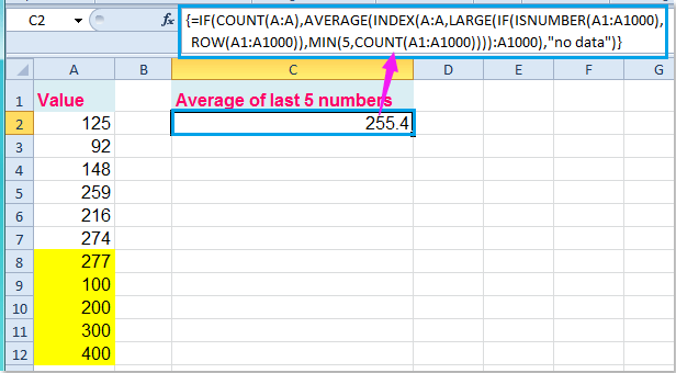
=IF(COUNT(A:A),AVERAGE(INDEX(A:A,LARGE(IF(ISNUMBER(A1:A10000),ROW(A1:A10000)),MIN(5,COUNT(A1:A10000)))):A10000),«no data») (A:A هو العمود الذي يحتوي على البيانات التي تستخدمها، وA1:A10000 نطاق ديناميكي يمكنك توسيعه حسب الحاجة، والرقم5 يشير إلى آخرn قيمة.) ثم اضغط على مفاتيحCtrl + Shift + Enter معًا للحصول على متوسط آخر 5 أرقام. راجع لقطة الشاشة:

الآن، عند إدخال أرقام جديدة بعد البيانات الأصلية، سيُحدَّث المتوسط تلقائيًا. راجع لقطة الشاشة:
ملاحظة: إذا كان عمود الخلايا يحتوي على قيم صفرية وترغب في استبعادها عند حساب متوسط آخر 5 قيم غير صفرية، فإن الصيغة السابقة لن تعمل. إليك صيغة مصفوفة بديلة لتحقيق ذلك—يرجى إدخالها:
=AVERAGE(SUBTOTAL(9,OFFSET(A1:A10000,LARGE(IF(A1:A10000>0,ROW(A1:A10000)-MIN(ROW(A1:A10000))),ROW(INDIRECT("1:5"))),0,1)))، ثم اضغط على مفاتيحCtrl + Shift + Enterللحصول على النتيجة التي تحتاجها، راجع لقطة الشاشة:

مقالات ذات صلة:
كيفية حساب متوسط كل 5 صفوف أو أعمدة في Excel؟
كيفية حساب متوسط أعلى أو أقل 3 قيم في Excel؟
أفضل أدوات الإنتاجية لمكتبتك
عزِّز مهاراتك في Excel باستخدام Kutools لـ Excel، وعايش الكفاءة كما لم تفعل من قبل.يقدّم Kutools لـ Excel أكثر من 300 ميزة متقدمة لتعزيز الإنتاجية ووقت الحفظ.انقر هنا للحصول على الميزة التي تحتاجها أكثر من غيرها...
يجلب Office Tab واجهة ذات علامات تبويب إلى Office، ويجعل عملك أسهل بكثير
- تمكّن من التحرير والقراءة باستخدام علامات التبويب في Word وExcel وPowerPoint، وPublisher وAccess وVisio وProject.
- افتح وأنشئ مستندات متعددة في علامات تبويب جديدة داخل النافذة نفسها، بدلاً من فتح نوافذ جديدة.
- يزيد إنتاجيتك بنسبة 50% ويوفّر لك مئات نقرات الفأرة كل يوم!
جميع الإضافات من Kutools في برنامج تثبيت واحد!
Kutools for Office حزمةٌ تحتوي على إضافاتٍ مخصصة لتطبيقات Excel وWord وOutlook وPowerPoint، إلى جانب Office Tab Pro، مما يجعلها الخيار المثالي للفِرق التي تعمل عبر تطبيقات Office.
- حزمة شاملة واحدة— إضافات Excel وWord وOutlook وPowerPoint بالإضافة إلى Office Tab Pro
- برنامج تثبيت واحد، ترخيص واحد— الإعداد خلال دقائق (جاهز لـ MSI)
- يعمل بشكل أفضل معًا— إنتاجية ميسَّرة عبر تطبيقات Office
- تجربة مجانية لمدة 30 يومًا بكامل الميزات— بدون تسجيل، بدون بطاقة ائتمان
- أفضل قيمة— وفِّر مقارنةً بشراء الإضافات بشكل منفصل