كيف يمكن الرجوع إلى اسم علامة التبويب من داخل خلية في Excel؟

للحصول على اسم علامة تبويب ورقة العمل الحالية في خلية بـ Excel، يمكنك استخدام صيغة أو دالة مُعرَّفة من قِبل المستخدم. سيأخذك هذا البرنامج التعليمي خلال الخطوات التالية.

الرجوع إلى اسم علامة التبويب ورقة العمل الحالية في الخلية باستخدام صيغة
الرجوع إلى اسم علامة التبويب ورقة العمل الحالية في الخلية باستخدام دالة معرّفة من قِبل المستخدم
الرجوع بسهولة إلى اسم علامة التبويب ورقة العمل الحالية في الخلية باستخدام Kutools لـ Excel

الرجوع إلى اسم علامة التبويب ورقة العمل الحالية في الخلية باستخدام صيغة

اتبع الخطوات التالية للرجوع إلى اسم علامة تبويب ورقة العمل الحالية في خلية معيّنة في Excel.

1. حدد خلية فارغة، ثم انسخ الصيغة التالية إليها:=MID(CELL(«filename»,A1),FIND(«]»,CELL(«filename»,A1))+1,255) في شريط الصيغة، واضغط بعد ذلك على مفتاحEnter. انظر لقطة الشاشة:

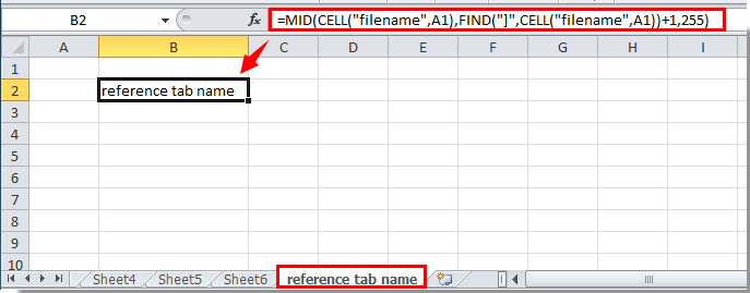
الآن، تم ربط اسم علامة تبويب الورقة بالخلية.

الرجوع إلى اسم علامة التبويب ورقة العمل الحالية في الخلية باستخدام دالة معرّفة من قِبل المستخدم

بالإضافة إلى الطريقة السابقة، يمكنك الرجوع إلى اسم علامة تبويب الورقة من داخل خلية باستخدام دالة مُعرَّفة من قِبل المستخدم.

1. اضغط علىAlt+F11 لفتح نافذةMicrosoft Visual Basic for Applications.

2. في نافذةMicrosoft Visual Basic for Applications، انقر علىInsert > Module. انظر لقطة الشاشة:

3. انقل الكود أدناه إلى نافذة الكود، ثم اضغط على مفاتيحAlt+Q لإغلاق نافذةMicrosoft Visual Basic for Applications.

كود VBA: الرجوع إلى اسم علامة التبويب

Function TabName()
  TabName = ActiveSheet.Name
End Function

4. انتقل إلى الخلية التي تريد أن يظهر فيها اسم علامة تبويب ورقة العمل الحالية، وأدخل الصيغة التالية: =TabName()، ثم اضغط على مفتاحEnter، وسيظهر اسم علامة تبويب ورقة العمل الحالية في الخلية.

الرجوع إلى اسم علامة التبويب ورقة العمل الحالية في الخلية باستخدام Kutools لـ Excel

باستخدام أداةإدراج معلومات ورقة العملمنKutools لـ Excel، يمكنك بسهولة الرجوع إلى اسم علامة تبويب الورقة في أي خلية تريدها. اتبع الخطوات التالية:

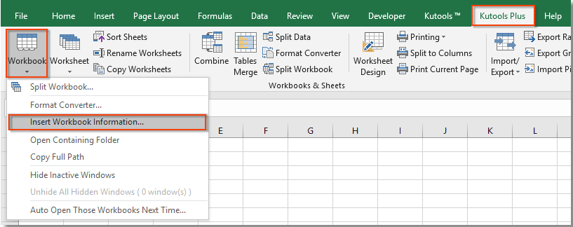
1. انقر علىKUTOOLS PLUS > Workbook > إدراج معلومات ورقة العمل. انظر لقطة الشاشة:

2. في مربع الحوارإدراج معلومات الورقة العمل، حدد الخياراسم ورقة العملضمن قسمInformation، وفي قسمInsert at، اخترRange، ثم حدد خلية فارغة لإدخال اسم الورقة فيها، وانقر أخيرًا على زرOK.

يمكنك ملاحظة أن اسم ورقة العمل الحالية قد تم الرجوع إليه في الخلية المحددة. انظر لقطة الشاشة:

عرض توضيحي: الرجوع بسهولة إلى اسم علامة التبويب ورقة العمل الحالية في الخلية باستخدام Kutools لـ Excel

Kutools لـ Excelتتضمّن أكثر من 300 أداة مفيدة لـ Excel! جرّبها مجانًا دون أي قيود لمدة 30 يومًا.حمّل النسخة التجريبية المجانية الآن!

أفضل أدوات الإنتاجية لمكتبتك

🤖	KUTOOLS AI مساعد: ثوّر تحليل البيانات استنادًا إلى:التنفيذ الذكي   |  إنشاء الكود|  إنشاء الصيغ المخصصة  |  تحليل البيانات وإنشاء المخططات البيانية|  استدعاء الوظائف المحسنة…
	الميزات الشائعة:البحث، التمييز أو وضع علامة على المكررات   |  حذف الصفوف الفارغة   |  دمج الأعمدة أو الخلايا دون فقدان البيانات   |  التقريب بدون استخدام الصيغة...
	بحث متقدم:VLookup متعدد المعايير  |  VLookup متعدد القيم  |   VLookup عبر أوراق متعددة   |   مطابقة غامضة....
	قائمة منسدلة متقدمة:إنشاء قائمة منسدلة بسرعة   |  قائمة منسدلة تابعة   |  قائمة منسدلة متعددة الاختيار....
	مدير الأعمدة:إضافة عدد محدد من الأعمدة|نقل الأعمدة|تبديل حالة ظهور الأعمدة المخفية|مقارنة النطاقات والأعمدة...
	ميزات مميزة:التركيز على الشبكة   |  عرض التصميم   |شريط الصيغ المحسن   | مدير الدفتر والورقة   |  مكتبة الموارد(نص تلقائي)|  أداة اختيار التاريخ   |  تجميع ورقات العمل  |  تشفير/فك تشفير الخلايا   | إرسال رسائل البريد الإلكتروني حسب القائمة   |  مرشح متقدم   |   تصفية خاصة(تصفية الخلايا التي تحتوي على خط عريض/مائل/يتوسطه خط...) ...
	أفضل 15 مجموعات الأدوات:12 أدواتالنصوص(إضافة نص،حذف الأحرف المحددة، ...)|   50+أنواعالمخططات البيانية(مخطط جانت، ...)|   40+ صيغعملية(حساب العمر بناءً على تاريخ الميلاد، ...)|   19 أدواتالإدراج(إدراج رمز QR،إدراج صورة من المسار، ...)|   12 أدواتالتحويل(تحويل إلى كلمات،تحويل العملة، ...)|   7 أدواتدمج وتقسيم(دمج متقدم للصفوف،تقسيم الخلايا، ...)|... وأكثر من ذلك

استخدم Kutools باللغة التي تفضلها – يدعم الإنجليزية والإسبانية والألمانية والفرنسية والصينية و40+ لغات أخرى!

عزِّز مهاراتك في Excel باستخدام Kutools لـ Excel، وعايش الكفاءة كما لم تفعل من قبل.يقدّم Kutools لـ Excel أكثر من 300 ميزة متقدمة لتعزيز الإنتاجية ووقت الحفظ.انقر هنا للحصول على الميزة التي تحتاجها أكثر من غيرها...

مزيد من التفاصيل حول Kutools لـ Excel...تنزيل مجاني...

---

يجلب Office Tab واجهة ذات علامات تبويب إلى Office، ويجعل عملك أسهل بكثير

• تمكّن من التحرير والقراءة باستخدام علامات التبويب في Word وExcel وPowerPoint، وPublisher وAccess وVisio وProject.
• افتح وأنشئ مستندات متعددة في علامات تبويب جديدة داخل النافذة نفسها، بدلاً من فتح نوافذ جديدة.
• يزيد إنتاجيتك بنسبة 50% ويوفّر لك مئات نقرات الفأرة كل يوم!

مزيد من التفاصيل حول Office Tab...تنزيل مجاني...

---

جميع الإضافات من Kutools في برنامج تثبيت واحد!

Kutools for Office حزمةٌ تحتوي على إضافاتٍ مخصصة لتطبيقات Excel وWord وOutlook وPowerPoint، إلى جانب Office Tab Pro، مما يجعلها الخيار المثالي للفِرق التي تعمل عبر تطبيقات Office.

• حزمة شاملة واحدة— إضافات Excel وWord وOutlook وPowerPoint بالإضافة إلى Office Tab Pro
• برنامج تثبيت واحد، ترخيص واحد— الإعداد خلال دقائق (جاهز لـ MSI)
• يعمل بشكل أفضل معًا— إنتاجية ميسَّرة عبر تطبيقات Office
• تجربة مجانية لمدة 30 يومًا بكامل الميزات— بدون تسجيل، بدون بطاقة ائتمان
• أفضل قيمة— وفِّر مقارنةً بشراء الإضافات بشكل منفصل

مزيد من التفاصيل حول Kutools for Office...تنزيل مجاني...