كيف تستخدم دالة VLOOKUP للعثور على أول قيمة مطابقة، أو الثانية، أو القيمة المطابقة n في Excel؟
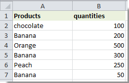
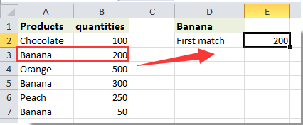
افترض أن لديك عمودين يحتويان على المنتجات والكميات كما في لقطة الشاشة أدناه. لمعرفة كميات الموز الأولى أو الثانية بسرعة، ماذا ستفعل؟
يمكنك هنا الاستفادة من دالة VLOOKUP لحل هذه المشكلة. في هذه المقالة، سنوضح لك كيفية استخدام دالة VLOOKUP في Excel للعثور على أول قيمة مطابقة، أو الثانية، أو القيمة المطابقة n.
استخدام VLOOKUP للعثور على أول قيمة مطابقة، أو الثانية، أو القيمة المطابقة n في Excel باستخدام صيغة
العثور بسهولة على أول قيمة مطابقة باستخدام VLOOKUP في Excel مع Kutools لـ Excel
استخدام VLOOKUP للعثور على أول قيمة مطابقة، أو الثانية، أو القيمة المطابقة n في Excel
يرجى اتباع الخطوات التالية للعثور على أول قيمة مطابقة، أو الثانية، أو القيمة المطابقة n في Excel.
1. في الخلية D1، أدخل المعيار الذي تريد البحث عنه باستخدام VLOOKUP—مثلًا، «موز».
2. سنبحث هنا عن أول قيمة مطابقة للموز. حدد خلية فارغة مثل E2، ثم انسخ الصيغة=INDEX($B$2:$B$6,MATCH(TRUE,EXACT($D$1,$A$2:$A$6),0)) والصقها في شريط الصيغة، ثم اضغط على مفاتيحCtrl+Shift+Enter معًا في آنٍ واحد.
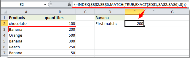
ملاحظة: في هذه الصيغة، يُعدّ $B$2:$B$6 نطاق القيم المطابقة، و$A$2:$A$6 هو النطاق الذي يحتوي على جميع معايير البحث المستخدمة مع VLOOKUP، بينما تمثّل الخلية $D$1 معيار VLOOKUP المحدد.
ستحصل بعد ذلك على أول قيمة مطابقة للموز في الخلية E2. وباستخدام هذه الصيغة، يمكنك استخراج أول قيمة مطابقة فقط وفقًا لمعيارك.
للحصول على القيمة المطابقة n، طبّق الصيغة التالية:=INDEX($B$2:$B$6,SMALL(IF($D$1=$A$2:$A$6,ROW($A$2:$A$6)-ROW($A$2)+1),1))، ثم اضغطCtrl+Shift+Enter معًا، وستُرجع هذه الصيغة أول قيمة مطابقة.
ملاحظات:
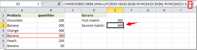
1. لإيجاد القيمة المطابقة الثانية، عدّل الصيغة أعلاه إلى=INDEX($B$2:$B$6,SMALL(IF($D$1=$A$2:$A$6,ROW($A$2:$A$6)-ROW($A$2)+1),2))، ثم اضغط على مفاتيحCtrl+Shift+Enter في آنٍ واحد. انظر لقطة الشاشة:
2. الرقم الأخير في الصيغة أعلاه يشير إلى القيمة المطابقة n لمعيار VLOOKUP. فإذا غيّرته إلى 3، فستحصل على القيمة المطابقة الثالثة، وإذا غيّرته إلى n، فستعثر على القيمة المطابقة n.
العثور على أول قيمة مطابقة باستخدام VLOOKUP في Excel مع Kutools لـ Excel
يمكنك العثور بسهولة على أول قيمة مطابقة في Excel دون الحاجة إلى حفظ الصيغ باستخدام صيغةالبحث عن البيانات في نطاقمنKutools لـ Excel.
قبل استخدامKutools لـ Excel، يُرجىتنزيله وتثبيته أولاً.
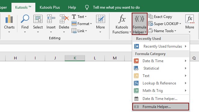
1. حدد خلية لوضع أول قيمة مطابقة فيها (مثل الخلية E2)، ثم انقر علىKutools > مساعد الصيغة > مساعد الصيغة. انظر لقطة الشاشة:
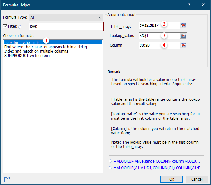
فيمساعد الصيغة، يُرجى التهيئة كما يلي:
- فيحدد صيغة، ابحث وحدّدالبحث عن البيانات في نطاق؛
نصائح: يمكنك تأشير خانةتصفية، ثم إدخال كلمة معيّنة في مربّع النص لتصفية الصيغ بسرعة. - فيمصفوفة_الجدول، حددالجدول الذي يحتوي على قيم التطابق الأولى.؛
- فيقيمة_البحث، حدد الخلية التي تحتوي علىالمعيارالذي ستعيد القيمة الأولى بناءً عليه؛
- فيالعمود، حدّد العمود الذي تريد استرداد القيمة المطابقة منه، أو يمكنك إدخال رقم العمود مباشرةً في مربع النص حسب حاجتك.
- انقر على زرموافق. انظر لقطة الشاشة:
الآن، سيتم ملء قيمة الخلية المقابلة تلقائيًا في الخلية C10 وفقًا لاختيارك من القائمة المنسدلة.
إذا كنت ترغب في تجربة هذه الأداة مجانًا (لمدة 30 يومًا)،فما عليك سوى النقر لتنزيلها، ثم اتبع الخطوات المذكورة أعلاه لتطبيق العملية.
أفضل أدوات الإنتاجية لمكتبتك
عزِّز مهاراتك في Excel باستخدام Kutools لـ Excel، وعايش الكفاءة كما لم تفعل من قبل.يقدّم Kutools لـ Excel أكثر من 300 ميزة متقدمة لتعزيز الإنتاجية ووقت الحفظ.انقر هنا للحصول على الميزة التي تحتاجها أكثر من غيرها...
يجلب Office Tab واجهة ذات علامات تبويب إلى Office، ويجعل عملك أسهل بكثير
- تمكّن من التحرير والقراءة باستخدام علامات التبويب في Word وExcel وPowerPoint، وPublisher وAccess وVisio وProject.
- افتح وأنشئ مستندات متعددة في علامات تبويب جديدة داخل النافذة نفسها، بدلاً من فتح نوافذ جديدة.
- يزيد إنتاجيتك بنسبة 50% ويوفّر لك مئات نقرات الفأرة كل يوم!
جميع الإضافات من Kutools في برنامج تثبيت واحد!
Kutools for Office حزمةٌ تحتوي على إضافاتٍ مخصصة لتطبيقات Excel وWord وOutlook وPowerPoint، إلى جانب Office Tab Pro، مما يجعلها الخيار المثالي للفِرق التي تعمل عبر تطبيقات Office.
- حزمة شاملة واحدة— إضافات Excel وWord وOutlook وPowerPoint بالإضافة إلى Office Tab Pro
- برنامج تثبيت واحد، ترخيص واحد— الإعداد خلال دقائق (جاهز لـ MSI)
- يعمل بشكل أفضل معًا— إنتاجية ميسَّرة عبر تطبيقات Office
- تجربة مجانية لمدة 30 يومًا بكامل الميزات— بدون تسجيل، بدون بطاقة ائتمان
- أفضل قيمة— وفِّر مقارنةً بشراء الإضافات بشكل منفصل