كيف يمكن استخدام دالة VLOOKUP لإرجاع قيم متعددة في خلية واحدة في Excel؟
تُعد دالة VLOOKUP أداةً قويةً في Excel، لكنها تُرجع افتراضيًا القيمة المطابقة الأولى فقط. فماذا لو احتجتَ استرداد **جميع** القيم المطابقة ودمجها في خلية واحدة؟ هذا طلب شائع جدًّا عند تحليل مجموعات البيانات أو تلخيص المعلومات. في هذا الدليل، سنرشدك خطوة بخطوة إلى طرق فعّالة لإرجاع قيم متعددة في خلية واحدة باستخدام الصيغ وميزة مفيدة.
إرجاع قيم متعددة في خلية واحدة باستخدام دالة TEXTJOIN (Excel 2019 وOffice 365)
إرجاع قيم متعددة في خلية واحدة باستخدام Kutools
إرجاع قيم متعددة في خلية واحدة باستخدام دالة معرّفة من قِبل المستخدم (User Defined Function)
إرجاع قيم متعددة في خلية واحدة باستخدام دالة TEXTJOIN (Excel 2019 وOffice 365)
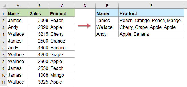
إذا كنت تستخدم إصدارًا أحدث من Excel، مثل Excel 2019 أو Office 365، فستجد دالة جديدة قوية تُسمىTEXTJOIN، تتيح لك بسرعة تنفيذ عملية بحث رأسي (VLOOKUP) وإرجاع جميع القيم المطابقة في خلية واحدة!
إرجاع جميع القيم المطابقة في خلية واحدة
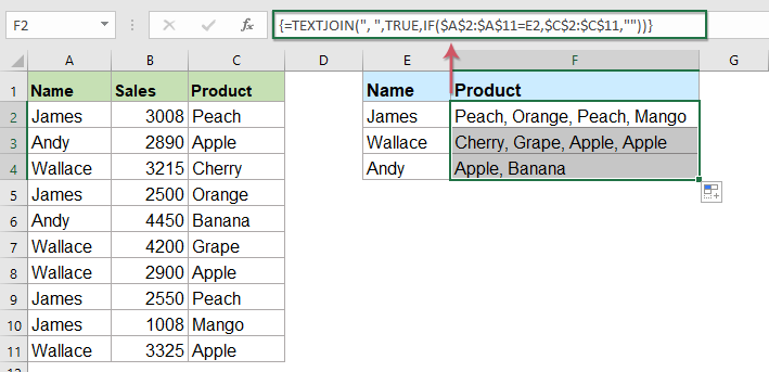
يرجى تطبيق الصيغة أدناه في خلية فارغة حيث تريد وضع النتيجة، ثم اضغط على مفاتيح Ctrl + Shift + Enter معًا للحصول على النتيجة الأولى، ثم اسحب مقبض التعبئة لأسفل حتى الخلية التي تريد استخدام هذه الصيغة فيها، وستحصل على جميع القيم المطابقة كما هو موضح في لقطة الشاشة أدناه:
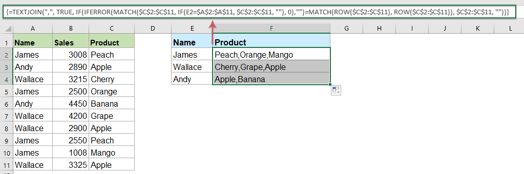
إرجاع جميع القيم المطابقة دون تكرار في خلية واحدة
إذا كنت ترغب في استرجاع جميع القيم المطابقة بناءً على بيانات البحث دون أي تكرار، فقد تكون الصيغة التالية مفيدة لك.
يرجى نسخ ولصق الصيغة التالية في خلية فارغة، ثم اضغط على مفاتيح Ctrl + Shift + Enter معًا للحصول على النتيجة الأولى، ثم انسخ هذه الصيغة لتعبئة الخلايا الأخرى، وستحصل على جميع القيم المطابقة دون التكرارات كما هو موضح في لقطة الشاشة أدناه:
إرجاع قيم متعددة في خلية واحدة باستخدام Kutools
باستخدام ميزة «دمج متقدم للصفوف» من Kutools لـ Excel، يمكنك بسهولة استرداد القيم المطابقة المتعددة في خلية واحدة—بدون الحاجة إلى صيغ معقدة! ودّع الحلول اليدوية واستكشف طريقة أكثر كفاءة للتعامل مع مهام البحث في Excel. دعنا نكتشف معًا كيف يمكّنك Kutools لـ Excel من إنجاز كل ذلك!
بعد تثبيت Kutools لـ Excel، يرجى اتباع الخطوات التالية:
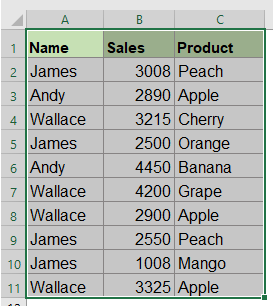
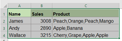
1. حدد نطاق البيانات الذي ترغب في دمج بيانات أحد أعمدته استنادًا إلى عمود آخر.
2. انقر على «Kutools» > «دمج وتقسيم» > «دمج متقدم للصفوف»، كما هو موضح في لقطة الشاشة التالية:

3. في مربع الحوار المنبثق «دمج الصفوف المتقدم»:
- انقر على اسم العمود الرئيسي الذي تريد الدمج بناءً عليه، ثم اختر «المفتاح الأساسي».
- ثم انقر على العمود الآخر الذي ترغب في دمج بياناته بناءً على العمود الرئيسي، وافتح القائمة المنسدلة من حقل «العملية»، واختر فاصلًا واحدًا لفصل البيانات المدمجة من قسم «الدمج».
- بعد ذلك، انقر على زر «موافق».

تم دمج جميع القيم المطابقة من عمود آخر، استنادًا إلى نفس القيمة، في خلية واحدة. راجع لقطات الشاشة:
 |  |
نصائح: إذا كنت تريد إزالة المحتوى المكرر أثناء دمج الخلايا، فما عليك سوى تحديد خيار «حذف القيم المكررة» في مربع الحوار. سيضمن لك ذلك دمج الإدخالات الفريدة فقط في خلية واحدة، مما يجعل بياناتك أكثر نظافة وتنظيمًا دون أي جهد إضافي. انظر لقطات الشاشة:
 |  |
حمّل Kutools لـ Excel وجربه مجانًا الآن!
إرجاع قيم متعددة في خلية واحدة باستخدام دالة معرّفة من قِبل المستخدم (User Defined Function)
دالة TEXTJOIN المذكورة أعلاه متوفرة فقط في Excel 2019 وOffice 365؛ لذا إذا كنت تستخدم إصدارًا أقدم من Excel، فستحتاج إلى استخدام بعض الأكواد لإتمام هذه المهمة.
إرجاع جميع القيم المطابقة في خلية واحدة
1. اضغط مع الاستمرار على مفاتيح «ALT + F11» لفتح نافذة «Microsoft Visual Basic for Applications».
2. انقر على «Insert» > «Module»، ثم الصق الكود التالي في نافذة الوحدة النمطية (Module Window).
كود VBA: بحث رأسي (Vlookup) لإرجاع قيم متعددة في خلية واحدة
Function ConcatenateIf(CriteriaRange As Range, Condition As Variant, ConcatenateRange As Range, Optional Separator As String = ",") As Variant
'Updateby Extendoffice
Dim xResult As String
On Error Resume Next
If CriteriaRange.Count <> ConcatenateRange.Count Then
    ConcatenateIf = CVErr(xlErrRef)
    Exit Function
End If
For i = 1 To CriteriaRange.Count
    If CriteriaRange.Cells(i).Value = Condition Then
        xResult = xResult & Separator & ConcatenateRange.Cells(i).Value
    End If
Next i
If xResult <> "" Then
    xResult = VBA.Mid(xResult, VBA.Len(Separator) + 1)
End If
ConcatenateIf = xResult
Exit Function
End Function
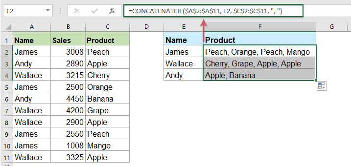
3. بعد ذلك، احفظ وأغلق هذا الكود، ثم عُد إلى ورقة العمل وأدخل الصيغة التالية: =CONCATENATEIF($A$2:$A$11, E2, $C$2:$C$11, ", ") في خلية فارغة محددة حيث تريد عرض النتيجة، ثم اسحب مقبض التعبئة لأسفل للحصول على جميع القيم المطابقة في خلية واحدة حسب رغبتك. انظر لقطة الشاشة:
إرجاع جميع القيم المطابقة دون تكرار في خلية واحدة
لتجاهل القيم المكررة في النتائج المطابقة، استخدم الكود أدناه.
1. اضغط مع الاستمرار على مفاتيح «Alt + F11» لفتح نافذة «Microsoft Visual Basic for Applications».
2. انقر على «Insert» > «Module»، ثم الصق الكود التالي في نافذة الوحدة النمطية (Module Window).
كود VBA: بحث رأسي (Vlookup) وإرجاع قيم مطابقة فريدة متعددة في خلية واحدة
Function MultipleLookupNoRept(Lookupvalue As String, LookupRange As Range, ColumnNumber As Integer)
'Updateby Extendoffice
    Dim xDic As New Dictionary
    Dim xRows As Long
    Dim xStr As String
    Dim i As Long
    On Error Resume Next
    xRows = LookupRange.Rows.Count
    For i = 1 To xRows
        If LookupRange.Columns(1).Cells(i).Value = Lookupvalue Then
            xDic.Add LookupRange.Columns(ColumnNumber).Cells(i).Value, ""
        End If
    Next
    xStr = ""
    MultipleLookupNoRept = xStr
    If xDic.Count > 0 Then
        For i = 0 To xDic.Count - 1
            xStr = xStr & xDic.Keys(i) & ","
        Next
        MultipleLookupNoRept = Left(xStr, Len(xStr) - 1)
    End If
End Function
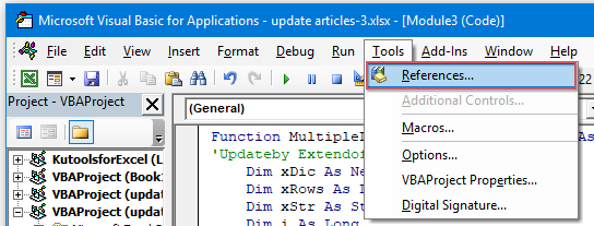
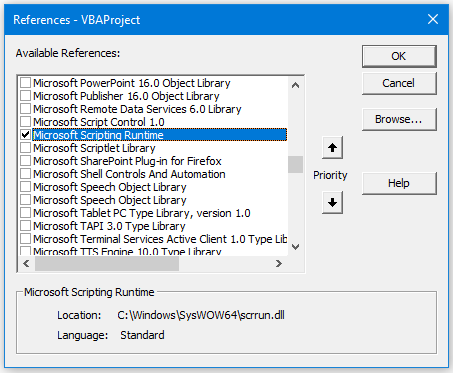
3. بعد إدراج الكود، انتقل إلى نافذة «Microsoft Visual Basic for Applications» المفتوحة، ثم انقر على «Tools» > «References». في مربع الحوار المنبثق «References – VBAProject»، حدد خيار «Microsoft Scripting Runtime» من قائمة «Available References». راجع لقطات الشاشة التالية:
 |  |
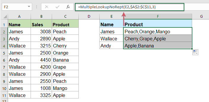
4. بعد ذلك، انقر على «موافق» لإغلاق مربع الحوار، ثم احفظ وأغلق نافذة الكود، وارجع إلى ورقة العمل. أدخل الصيغة التالية: =MultipleLookupNoRept(E2,$A$2:$C$11,3) في خلية فارغة حيث تريد عرض النتيجة، ثم اسحب مقبض التعبئة لأسفل للحصول على جميع القيم المطابقة. انظر لقطة الشاشة:
سواء اخترت استخدام صيغ مثل TEXTJOIN مع دوال صفيفية، أو الاعتماد على أدوات مثل Kutools لـ Excel أو دالة مُعرَّفة من قِبل المستخدم، فإن جميع هذه الطرق تُسهّل عليك تنفيذ مهام البحث المعقدة. اختر الطريقة الأنسب لاحتياجاتك! وإذا كنت مهتمًّا باستكشاف المزيد من نصائح وحيل Excel،يقدّم موقعنا آلاف البرامج التعليمية.
مقالات ذات صلة إضافية:
- دالة VLOOKUP مع أمثلة أساسية ومتقدمة
- في Excel، تُعد دالة VLOOKUP أداةً قويةً يعتمد عليها معظم المستخدمين للبحث عن قيمة موجودة في العمود الأقصى يسارًا ضمن نطاق البيانات، ثم إرجاع القيمة المقابلة لها من عمودٍ تحدده أنت في نفس الصف. ويستعرض هذا البرنامج التعليمي كيفية استخدام دالة VLOOKUP عبر أمثلة أساسية ومتقدمة في Excel.
- إرجاع قيم متعددة مطابقة بناءً على معيار واحد أو أكثر
- عادةً ما يكون البحث عن قيمة محددة وإرجاع العنصر المطابق أمرًا سهلًا لمعظمنا باستخدام دالة VLOOKUP. لكن، هل سبق أن حاولت إرجاع قيم متعددة مطابقة بناءً على معيار واحد أو أكثر؟ في هذه المقالة، سأقدّم لك بعض الصيغ الفعّالة لحل هذه المهمة المعقدة في Excel.
- البحث الرأسي (Vlookup) وإرجاع قيم متعددة رأسيًّا
- عادةً، تُستخدم دالة VLOOKUP للحصول على أول قيمة مطابقة، لكن في بعض الأحيان قد ترغب في استرجاع جميع السجلات المطابقة وفقًا لمعيار معيّن. في هذه المقالة، سأوضح لك كيفية تنفيذ بحث رأسي (VLOOKUP) لإرجاع جميع القيم المطابقة—سواء رأسيًّا أو أفقيًّا أو حتى داخل خلية واحدة.
- البحث الرأسي (Vlookup) وإرجاع قيم متعددة من قائمة منسدلة
- في Excel، كيف يمكنك تنفيذ عملية بحث رأسي (VLOOKUP) لإرجاع جميع القيم المطابقة دفعةً واحدة من قائمة منسدلة؟ أي أنه عند اختيارك عنصرًا من القائمة، تظهر فورًا كل القيم المرتبطة به. في هذه المقالة، سأعرض لك الحل خطوة بخطوة.
أفضل أدوات الإنتاجية لمكتبتك
عزِّز مهاراتك في Excel باستخدام Kutools لـ Excel، وعايش الكفاءة كما لم تفعل من قبل.يقدّم Kutools لـ Excel أكثر من 300 ميزة متقدمة لتعزيز الإنتاجية ووقت الحفظ.انقر هنا للحصول على الميزة التي تحتاجها أكثر من غيرها...
يجلب Office Tab واجهة ذات علامات تبويب إلى Office، ويجعل عملك أسهل بكثير
- تمكّن من التحرير والقراءة باستخدام علامات التبويب في Word وExcel وPowerPoint، وPublisher وAccess وVisio وProject.
- افتح وأنشئ مستندات متعددة في علامات تبويب جديدة داخل النافذة نفسها، بدلاً من فتح نوافذ جديدة.
- يزيد إنتاجيتك بنسبة 50% ويوفّر لك مئات نقرات الفأرة كل يوم!
جميع الإضافات من Kutools في برنامج تثبيت واحد!
Kutools for Office حزمةٌ تحتوي على إضافاتٍ مخصصة لتطبيقات Excel وWord وOutlook وPowerPoint، إلى جانب Office Tab Pro، مما يجعلها الخيار المثالي للفِرق التي تعمل عبر تطبيقات Office.
- حزمة شاملة واحدة— إضافات Excel وWord وOutlook وPowerPoint بالإضافة إلى Office Tab Pro
- برنامج تثبيت واحد، ترخيص واحد— الإعداد خلال دقائق (جاهز لـ MSI)
- يعمل بشكل أفضل معًا— إنتاجية ميسَّرة عبر تطبيقات Office
- تجربة مجانية لمدة 30 يومًا بكامل الميزات— بدون تسجيل، بدون بطاقة ائتمان
- أفضل قيمة— وفِّر مقارنةً بشراء الإضافات بشكل منفصل