كيف تُفرز البيانات الأبجدية الرقمية التي تبدأ بأرقام في Excel؟
إذا كانت بياناتك في Excel تحتوي على إدخالات تبدأ بأرقام متبوعة بنص اختياري (مثل "201510"، "201510AA"، "201520")، فقد لا يُنتج الفرز المباشر الترتيب الذي تريده. عادةً ما يفصل Excel بين القيم الرقمية البحتة والقيم الأبجدية الرقمية، مما قد يؤدي إلى تسلسل غير منطقي—فمثلًا، قد يُفرَز "201510" بشكل منفصل عن "201510AA". يوضح هذا الدليل كيفية فرز هذه البيانات الأبجدية الرقمية مع الحفاظ على ترتيب البادئات الرقمية بشكل صحيح، لضمان ظهور النتائج بالشكل المطلوب: "201510"، "201510AA"، "201520".
فرز البيانات الأبجدية الرقمية باستخدام عمود مساعد الصيغة
| البيانات الأصلية | نتيجة الفرز العادية | نتيجة الفرز المطلوبة منك | ||
 |  |  | |  |
 فرز البيانات الأبجدية الرقمية باستخدام عمود مساعد الصيغة
في Excel، يمكنك إنشاء عمود مساعد الصيغة، ثم فرز البيانات وفقًا لهذا العمود الجديد، يُرجى اتباع الخطوات التالية:
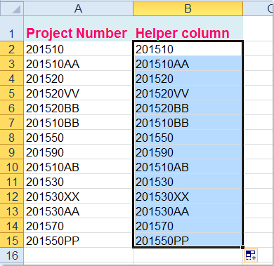
1. أدخل هذه الصيغة=TEXT(A2, «###») في خلية فارغة بجانب بياناتك، مثل B2، كما هو موضح في لقطة الشاشة:

2. بعد ذلك، اسحب مقبض التعبئة لأسفل إلى الخلايا التي ترغب في تطبيق الصيغة عليها، كما هو موضح في لقطة الشاشة:
3. بعد ذلك، قم بفرز البيانات وفقًا للعمود الجديد: حدد عمود المساعدة الذي أنشأته، ثم انقر فوقبيانات > فرز. في مربع الحوار المنبثق، اخترتوسيع التحديد، كما هو موضح في لقطات الشاشة:
 | |  |
4. ثم انقر فوق زرفرزلفتح مربع حوارفرز. ضمن قسمالعمود، اختر اسمعمود المساعدةالذي تريد الفرز وفقًا له، واستخدمالقيمفي قسمفرز حسب، ثم حدد ترتيب الفرز الذي تريده، كما هو موضح في لقطة الشاشة:

5. ثم انقر فوقموافق، وفي مربع تحذير الفرز المنبثق، يرجى تحديدفرز الأرقام والأرقام المخزَّنة كنص بشكل منفصل، كما هو موضح في لقطة الشاشة:

6. ثم انقر فوق زرموافق، وسترى الآن أن البيانات قد تم فرزها بالضبط كما تحتاج!

7. في النهاية، يمكنك حذف محتويات عمود المساعدة متى شئت.
أفضل أدوات الإنتاجية لمكتبتك
عزِّز مهاراتك في Excel باستخدام Kutools لـ Excel، وعايش الكفاءة كما لم تفعل من قبل.يقدّم Kutools لـ Excel أكثر من 300 ميزة متقدمة لتعزيز الإنتاجية ووقت الحفظ.انقر هنا للحصول على الميزة التي تحتاجها أكثر من غيرها...
يجلب Office Tab واجهة ذات علامات تبويب إلى Office، ويجعل عملك أسهل بكثير
- تمكّن من التحرير والقراءة باستخدام علامات التبويب في Word وExcel وPowerPoint، وPublisher وAccess وVisio وProject.
- افتح وأنشئ مستندات متعددة في علامات تبويب جديدة داخل النافذة نفسها، بدلاً من فتح نوافذ جديدة.
- يزيد إنتاجيتك بنسبة 50% ويوفّر لك مئات نقرات الفأرة كل يوم!
جميع الإضافات من Kutools في برنامج تثبيت واحد!
Kutools for Office حزمةٌ تحتوي على إضافاتٍ مخصصة لتطبيقات Excel وWord وOutlook وPowerPoint، إلى جانب Office Tab Pro، مما يجعلها الخيار المثالي للفِرق التي تعمل عبر تطبيقات Office.
- حزمة شاملة واحدة— إضافات Excel وWord وOutlook وPowerPoint بالإضافة إلى Office Tab Pro
- برنامج تثبيت واحد، ترخيص واحد— الإعداد خلال دقائق (جاهز لـ MSI)
- يعمل بشكل أفضل معًا— إنتاجية ميسَّرة عبر تطبيقات Office
- تجربة مجانية لمدة 30 يومًا بكامل الميزات— بدون تسجيل، بدون بطاقة ائتمان
- أفضل قيمة— وفِّر مقارنةً بشراء الإضافات بشكل منفصل