كيف تُجري بحثًا رأسيًّا (VLOOKUP) وتدمج القيم المطابقة المتعددة في إكسل؟
عند استخدام دالة VLOOKUP في إكسل، فإنها عادةً ما تُعيد أول قيمة مطابقة فقط وفقًا لمعيار البحث. لكن في العديد من السيناريوهات الشائعة، قد تحتاج إلى استرداد ودمج **جميع** القيم المطابقة المرتبطة بمفتاح معين—مثل سرد جميع الطلاب في صف دراسي أو كل المنتجات التابعة لفئة معيّنة. وبما أن دالة VLOOKUP القياسية لا تدعم هذا السلوك بشكل افتراضي، فقد تتساءل: كيف يمكنك تنفيذ بحثٍ عمودي يجمع كل النتائج المطابقة في خلية واحدة؟ فيما يلي، سنستعرض عدة طرق عملية وفعّالة لتحقيق هذه المهمة، وتتناسب مع مختلف إصدارات إكسل وتفضيلات المستخدمين.
البحث الرأسي (Vlookup) ودمج القيم المطابقة المتعددة في إكسل
البحث الرأسي ودمج القيم المطابقة المتعددة باستخدام دالتي TEXTJOIN وFILTER
إذا كنت تستخدم Excel 365 أو Excel 2021، فإن الجمع بين دالتي TEXTJOIN وFILTER يوفّر حلاً فعّالًا قائمًا على الصيغة للبحث الرأسي ودمج جميع القيم المطابقة. وهو مثالي خصوصًا لمجموعات البيانات الديناميكية والمحدَّثة، حيث يتجدَّد الناتج تلقائيًا بمجرد تغيُّر البيانات الأصلية. ويُعد هذا الأسلوب الأنسب عندما يدعم إصدار Excel الخاص بك دالة FILTER، المتاحة حصريًّا في إصدارات Office الحديثة.
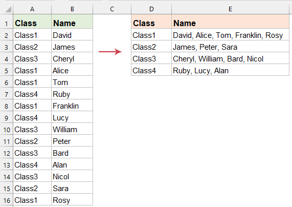
في الخلية المستهدفة، أدخل الصيغة التالية، ثم اسحبها لأسفل إذا رغبت في تطبيقها على صفوف أخرى أيضًا. سيتم استخراج جميع القيم المطابقة ودمجها تلقائيًا في خلية واحدة. انظر لقطة الشاشة:
=TEXTJOIN(", ", TRUE, FILTER($B$2:$B$16, $A$2:$A$16=D2, ""))
- FILTER($B$2:$B$16, $A$2:$A$16=D2, «»)يتحقق هذا الجزء من الصيغة من كل قيمة في النطاق $A$2:$A$16، وإذا تطابقت مع القيمة الموجودة في الخلية D2، فسيتم تضمين القيمة المقابلة لها من النطاق $B$2:$B$16 في مصفوفة النتائج.
- $B$2:$B$16النطاق الذي سيتم استرداد القيم المطابقة منه.
- $A$2:$A$16=D2الشرط الذي يُحدد وفقه اختيار القيم هو معالجة الصفوف التي تكون فيها القيم في النطاق $A$2:$A$16 مساوية للمحتوى الموجود في الخلية D2 فقط.
- TEXTJOIN(", ", TRUE, ...): تستلم هذه الدالة مخرجات دالة FILTER (وهي مصفوفة من القيم المطابقة)، وتقوم بدمجها في سلسلة نصية واحدة، مفصولة بالفاصل المحدد (فاصلة ومسافة)، مع تجاهل الإدخالات الفارغة تلقائيًا.
- ",": يعيّن الفاصلة متبوعةً بمسافة كفاصل؛ ويمكنك تغيير هذا الرمز حسب الحاجة، مثل استخدام الفواصل المنقوطة أو فواصل الأسطر.
- TRUE: يتجاهل الخلايا الفارغة تلقائيًا أثناء الدمج، ليمنحك ناتجًا منسقًا وأنيقًا.
ملاحظة خاصة: تتطلب هذه الطريقة Excel 365 أو 2021، ولا تعمل مع الإصدارات الأقدم (مثل Excel 2019 و2016 أو ما قبلها). تأكد دائمًا من إصدار Excel الخاص بك قبل البدء.
تلميح: إذا تغيّرت قيمة البحث (مثل D2) أو أُضيفت عناصر مطابقة جديدة إلى نطاق البيانات، فسيتم تحديث الناتج تلقائيًا دون الحاجة إلى أي خطوات إضافية.
القيود المحتملة: قد يزداد وقت حساب الصيغة عند التعامل مع مجموعات بيانات ضخمة جدًّا. كما يجب على المستخدمين التأكد من أن نطاقات البحث أو النتائج خالية من الخلايا المدمجة، إذ قد يؤدي وجودها إلى أخطاء في الصيغة.
البحث الرأسي ودمج القيم المطابقة المتعددة باستخدام Kutools لـ Excel
إذا وجدت أن الصيغ المدمجة معقدة أو أن إصدار Excel الخاص بك لا يدعم دوال متقدمة مثل TEXTJOIN وFILTER، فإن Kutools لـ Excel يقدم لك حلاً رسوميًا سهل الاستخدام. تتيح لك ميزة «بحث واحد إلى العديد» في Kutools تنفيذ البحث الرأسي ودمج جميع النتائج المطابقة في بضع خطوات بسيطة، مما يجعلها مثالية للمبتدئين والمستخدمين المتقدمين على حدٍّ سواء. مع Kutools، لن تحتاج إلى كتابة صيغ أو أكواد معقدة، خاصةً عند التعامل مع مجموعات بيانات كبيرة أو متغيرة تتطلب عمليات بحث وترحيل متكررة.
بعد تثبيت Kutools لـ Excel، اتبع الخطوات التالية:
انقرKutools > بحث متقدم > بحث واحد إلى العديد (إرجاع نتائج متعددة)لفتح مربع حوار الإعداد. ضمن هذا المربع، يمكنك تهيئة إعدادات البحث والإخراج بسرعة باستخدام الخطوات التالية:
- حدد خلايا الإخراج المستهدفة للنتائج المدمجة، والخلايا التي تحتوي على القيم التي ترغب في البحث عنها؛
- حدّد نطاق الجدول الذي يحتوي على عمود مفتاح البحث وعمود النتائج معًا؛
- عيّن العمود الذي يحتوي على مفاتيح البحث (العمود الرئيسي) والعمود الذي سيتم دمج قيمه (عمود الإرجاع)؛
- انقر على زر «موافق» لتأكيد إعداداتك ومعالجة البيانات.


النتيجة: سيعرض Kutools الآن جميع القيم المطابقة والمدمجة في خلية الإخراج المحددة. انظر لقطة الشاشة:
يُوصى بشدة بهذه الطريقة للمستخدمين الذين يفضلون العمل من واجهة إكسل دون الحاجة إلى صيغ أو أكواد معقدة، إذ تقلل من احتمالية وقوع أخطاء في الصيغ وتعزز الإنتاجية عند تنفيذ مهام البحث والدمج المتكررة.
البحث الرأسي ودمج القيم المطابقة المتعددة باستخدام دالة معرّفة من قبل المستخدم
للمستخدمين الماهرين في VBA (Visual Basic for Applications)، أو لأولئك الذين يستخدمون إصدارات قديمة من إكسل لا تدعم المصفوفات الديناميكية أو دالة FILTER، يمكنكم إنشاء دالة مخصصة معرّفة من قِبَل المستخدم (UDF) لتحقيق دمجٍ مرن للنتائج المتعددة. هذه الطريقة متوافقة عالميًّا مع جميع إصدارات إكسل، ويمكن تكييفها بسهولة مع رموز فواصل أو شروط محددة.
1. اضغط مع الاستمرار على مفاتيحALT + F11 لفتح نافذةمايكروسوفت فيجوال بيسك للتطبيقات.
2. انقرإدراج > وحدة نمطية (Module)، ثم الصق الكود التالي في نافذة الوحدة النمطية.
كود VBA: البحث الرأسي ودمج القيم المطابقة المتعددة في خلية
Function ConcatenateMatches(LookupValue As String, LookupRange As Range, ReturnRange As Range, Optional Delimiter As String = ", ") As String
'Updateby Extendoffice
    Dim Cell As Range
    Dim Result As String
    Result = ""
    For Each Cell In LookupRange
        If Cell.Value = LookupValue Then
            Result = Result & Cell.Offset(0, ReturnRange.Column - LookupRange.Column).Value & Delimiter
        End If
    Next Cell
    If Result <> "" Then
        Result = Left(Result, Len(Result) - Len(Delimiter))
    End If
    ConcatenateMatches = Result
End Function
3. احفظ وأغلق محرر VBA. عُد إلى ورقة العمل الخاصة بك، ثم استخدم الدالة المخصصة هذه بإدخال الصيغة التالية في خلية فارغة حيث تريد ظهور الناتج: =ConcatenateMatches(D2, $A$2:$A$16, $B$2:$B$16). اسحب مقبض التعبئة لأسفل لنسخ الصيغة إلى الخلايا الأخرى حسب الحاجة. سيتم جمع جميع القيم المطابقة بناءً على قيمة البحث المحددة ودمجها في خلية واحدة، مفصَّلة بفاصلة ومسافة. راجع لقطة الشاشة التالية:

- D2: القيمة التي تريد البحث عنها ومطابقتها داخل مجموعة البيانات الخاصة بك (LookupValue).
- A2:A16: النطاق الذي تبحث فيه الدالة عن قيمة البحث (LookupRange).
- B2:B16: النطاق الذي يحتوي على القيم التي سيتم دمجها عند تطابق قيمة البحث (ReturnRange).
البحث الرأسي ودمج القيم المطابقة المتعددة باستخدام كود VBA
بالنسبة للسيناريوهات التي تتطلب استخدامًا متكررًا أو للمستخدمين الراغبين في تجنّب دوال مخصصة في خلايا ورقة العمل، يُمكنك الاعتماد على ماكرو VBA جاهز لدمج النتائج مباشرةً—وهو حلٌّ فعّال جدًّا في البيئات المشتركة التي قد لا يمتلك فيها جميع المستخدمين نفس الإصدار أو الملحقات.
1. انقرأدوات المطور > فيجوال بيسكلفتح محرر VBA.
2. في نافذة VBA، انقرإدراج > وحدة نمطية (Module)، ثم الصق هذا الكود في الوحدة النمطية:
Sub VLookupAndConcatenate()
    Dim ws As Worksheet
    Dim dataRange As Range, lookupRange As Range, resultRange As Range
    Dim dict As Object
    Dim i As Long, lastRow As Long
    Dim lookupValue As Variant, result As String
    Dim delimiter As String
    delimiter = ", "
    Set dict = CreateObject("Scripting.Dictionary")
    Set ws = ActiveSheet
    On Error Resume Next
    Set dataRange = Application.InputBox( _
        Prompt:="Please select the data range (contains lookup column and result column)", _
        Title:="Select Data Range", _
        Type:=8)
    On Error GoTo 0
    If dataRange Is Nothing Then Exit Sub
    On Error Resume Next
    Set lookupRange = Application.InputBox( _
        Prompt:="Please select the lookup range (single column)", _
        Title:="Select Lookup Range", _
        Type:=8)
    On Error GoTo 0
    If lookupRange Is Nothing Then Exit Sub
    On Error Resume Next
    Set resultRange = Application.InputBox( _
        Prompt:="Please select the starting cell for results output", _
        Title:="Select Output Location", _
        Type:=8)
    On Error GoTo 0
    If resultRange Is Nothing Then Exit Sub
    resultRange.Resize(lookupRange.Rows.Count, 1).ClearContents
    For i = 1 To dataRange.Rows.Count
        lookupValue = dataRange.Cells(i, 1).Value
        If Not dict.Exists(lookupValue) Then
            dict.Add lookupValue, dataRange.Cells(i, 2).Value
        Else
            dict(lookupValue) = dict(lookupValue) & delimiter & dataRange.Cells(i, 2).Value
        End If
    Next i
    For i = 1 To lookupRange.Rows.Count
        lookupValue = lookupRange.Cells(i, 1).Value
        If dict.Exists(lookupValue) Then
            resultRange.Cells(i, 1).Value = dict(lookupValue)
        Else
            resultRange.Cells(i, 1).Value = "Not Found"
        End If
    Next i
    MsgBox "Operation completed! Processed " & lookupRange.Rows.Count & " lookup values.", vbInformation
End Sub
3. انقر على زر![]() لتشغيل الماكرو. ستظهر مربعات إدخال تطلب منك تحديد نطاق البيانات، ونطاق البحث، ونطاق النتائج. وبعد ذلك، سيتم عرض الناتج المدمج مباشرةً في خلايا الإخراج المحددة.
لتشغيل الماكرو. ستظهر مربعات إدخال تطلب منك تحديد نطاق البيانات، ونطاق البحث، ونطاق النتائج. وبعد ذلك، سيتم عرض الناتج المدمج مباشرةً في خلايا الإخراج المحددة.
يُعد هذا النهج القائم على الماكرو مفيدًا بشكل خاص إذا كنت تُجري بشكل متكرر عمليات بحث ودمج متعددة باستخدام قيم مختلفة، إذ يجنّبك تشويش ورقة العمل باستدعاءات الدوال المخصصة.
يمكنك بسهولة تعديل الفاصل في الكود عند الحاجة، وتوسيع الماكرو لإخراج النتائج إلى خلية أو ملف بما يتناسب مع سير عملك.
يمكنك دمج القيم المتقابلة المتعددة في إكسل باستخدام طرق متنوعة، لكلٍّ منها مزايا محددة تتناسب مع حالتك الخاصة. سواء اخترت صيغ المصفوفات الديناميكية، أو وظائف الإضافة مثل Kutools لـ Excel، أو الحلول القائمة على VBA، فإنك ستعزز قدرتك على تحليل البيانات المجمعة وعرضها بكفاءة أعلى. وبناءً على حجم مجموعة البيانات وتعقيدها، اختر الطريقة التي توفّر لك — أو لفريقك — أفضل أداءً وسهولةً في الصيانة. ولضمان أفضل النتائج في العمليات اليومية، تحقّق من اتساق البيانات، وتجنّب الدمج غير الضروري، وتأكد من صحة نطاقات المرجعيات. وإذا واجهت أخطاءً في حسابات الصيغ، فراجع مرةً أخرى أن نطاقاتك تتطابق مع البيانات وأنك تستخدم طريقة إدخال الصيغة المناسبة لإصدار إكسل الذي تعمل عليه.
للحصول على تقنيات إكسل متقدمة ومجموعة واسعة من أدلة الشرح العملية،قم بزيارة مكتبتنا الشاملة للدروس التعليمية.
أفضل أدوات الإنتاجية لمكتبتك
عزِّز مهاراتك في Excel باستخدام Kutools لـ Excel، وعايش الكفاءة كما لم تفعل من قبل.يقدّم Kutools لـ Excel أكثر من 300 ميزة متقدمة لتعزيز الإنتاجية ووقت الحفظ.انقر هنا للحصول على الميزة التي تحتاجها أكثر من غيرها...
يجلب Office Tab واجهة ذات علامات تبويب إلى Office، ويجعل عملك أسهل بكثير
- تمكّن من التحرير والقراءة باستخدام علامات التبويب في Word وExcel وPowerPoint، وPublisher وAccess وVisio وProject.
- افتح وأنشئ مستندات متعددة في علامات تبويب جديدة داخل النافذة نفسها، بدلاً من فتح نوافذ جديدة.
- يزيد إنتاجيتك بنسبة 50% ويوفّر لك مئات نقرات الفأرة كل يوم!
جميع الإضافات من Kutools في برنامج تثبيت واحد!
Kutools for Office حزمةٌ تحتوي على إضافاتٍ مخصصة لتطبيقات Excel وWord وOutlook وPowerPoint، إلى جانب Office Tab Pro، مما يجعلها الخيار المثالي للفِرق التي تعمل عبر تطبيقات Office.
- حزمة شاملة واحدة— إضافات Excel وWord وOutlook وPowerPoint بالإضافة إلى Office Tab Pro
- برنامج تثبيت واحد، ترخيص واحد— الإعداد خلال دقائق (جاهز لـ MSI)
- يعمل بشكل أفضل معًا— إنتاجية ميسَّرة عبر تطبيقات Office
- تجربة مجانية لمدة 30 يومًا بكامل الميزات— بدون تسجيل، بدون بطاقة ائتمان
- أفضل قيمة— وفِّر مقارنةً بشراء الإضافات بشكل منفصل