استخراج القيم الفريدة بناءً على معيار واحد أو أكثر في Excel
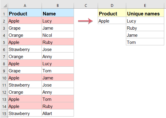
يُعد استخراج القيم الفريدة وفقًا لمعايير معيّنة خطوةً أساسية في تحليل البيانات وإعداد التقارير. تخيل أن لديك نطاق البيانات على اليسار، وترغب في عرض أسماء فريدة من العمود B فقط بناءً على معيار محدَّد في العمود A. سواء كنت تستخدم إصدارات Excel القديمة أو تستفيد من أحدث الميزات في Excel 365/2021، سيُرشدك هذا الدليل إلى كيفية استخراج القيم الفريدة بكفاءة وسلاسة.
استخراج القيم الفريدة بناءً على معايير في Excel
- باستخدام صيغة مصفوفة
- باستخدام Kutools لـ Excel
- باستخدام صيغة (Excel 365، Excel 2021 والإصدارات الأحدث)
استخراج القيم الفريدة بناءً على معايير متعددة في Excel
استخراج القيم الفريدة من قائمة خلايا باستخدام Kutools لـ Excel
استخراج القيم الفريدة بناءً على معايير في Excel
•باستخدام صيغة مصفوفة لعرض القيم الفريدة عموديًا
لحل هذه المهمة، يمكنك تطبيق صيغة مصفوفة معقدة، يُرجى اتباع الخطوات التالية:
1. أدخل الصيغة أدناه في خلية فارغة حيث تريد عرض نتيجة الاستخراج—في هذا المثال، سأضعها في الخلية E2—ثم اضغط على مفاتيح Shift + Ctrl + Enter للحصول على أول قيمة فريدة.
=IFERROR(INDEX($B$2:$B$15, MATCH(0, IF($D$2=$A$2:$A$15, COUNTIF($E$1:$E1, $B$2:$B$15), ""), 0)),"")2. بعد ذلك، اسحب مقبض التعبئة لأسفل حتى تظهر خلايا فارغة؛ وبذلك يتم عرض جميع القيم الفريدة وفقًا للمعيار المحدد. انظر لقطة الشاشة:

•استخراج وعرض القيم الفريدة في خلية واحدة باستخدام Kutools لـ Excel
يوفّر Kutools لـ Excel طريقةً مباشرةً لاستخراج القيم الفريدة وعرضها في خلية واحدة، مما يوفّر لك الوقت والجهد عند التعامل مع مجموعات بيانات كبيرة—بدون الحاجة إلى تذكّر أي صيغ!
بعد تثبيت Kutools لـ Excel، يُرجى اتباع ما يلي:
انقر على «Kutools» > «بحث متقدم» > «بحث واحد إلى العديد (تُرجع نتائج متعددة)» لفتح مربع الحوار. ثم في مربع الحوار، يُرجى تحديد العمليات على النحو التالي:
- اختر «منطقة وضع القائمة» و«نطاق قيمة البحث» في مربعَي النص بشكل منفصل؛
- اختر نطاق الجدول الذي تريد استخدامه؛
- حدّد العمود الرئيسي وعمود الإرجاع من القائمتَين المنسدلتَين «العمود الرئيسي» و«عمود الإرجاع» بشكل منفصل؛
- وأخيرًا، انقر على زر «موافق».


النتيجة:
تم استخراج جميع الأسماء الفريدة بناءً على المعيار في خلية واحدة، انظر لقطة الشاشة:
•باستخدام صيغة في Excel 365، Excel 2021 والإصدارات الأحدث لعرض القيم الفريدة عموديًا
مع Excel 365 وExcel 2021، تُبسّط الدوال مثل UNIQUE وFILTER عملية استخراج القيم الفريدة بشكل كبير.
أدخل الصيغة أدناه في خلية فارغة، ثم اضغط على مفتاح Enter للحصول على جميع الأسماء الفريدة دفعة واحدة مرتبة عموديًا.
=UNIQUE(FILTER(B2:B15, A2:A15=D2))
- FILTER(B2:B15, A2:A15=D2):
- FILTERيُرشّح البيانات من النطاق B2:B15.
- A2:A15=D2يتحقّق من الموضع الذي تتطابق فيه القيم في النطاق A2:A15 مع القيمة الموجودة في الخلية D2، ويتم تضمين الصفوف التي تستوفي هذا الشرط فقط في النتيجة.
- UNIQUE(...):
يضمن إرجاع القيم الفريدة فقط من بين نتائج التصفية.
استخراج القيم الفريدة بناءً على معايير متعددة في Excel
•باستخدام صيغة مصفوفة لعرض القيم الفريدة عموديًا
إذا أردت استخراج القيم الفريدة بناءً على شرطين، فهناك صيغة مصفوفة أخرى يمكن أن تساعدك، يُرجى اتباع ما يلي:
1. أدخل الصيغة أدناه في خلية فارغة حيث تريد عرض القيم الفريدة—في هذا المثال، سأضعها في الخلية G2—ثم اضغط على مفاتيح Shift + Ctrl + Enter للحصول على أول قيمة فريدة.
=IFERROR(INDEX($C$2:$C$15,MATCH(0,COUNTIF(G1:$G$1,$C$2:$C$15)+IF($A$2:$A$15<>$E$2,1,0)+IF($B$2:$B$15<>$F$2,1,0),0)),"")2. بعد ذلك، اسحب مقبض التعبئة لأسفل حتى تظهر خلايا فارغة؛ وبذلك يتم عرض جميع القيم الفريدة استنادًا إلى الشرطين المحددين. انظر لقطة الشاشة:

•باستخدام في Excel 365، Excel 2021 والإصدارات الأحدث لعرض القيم الفريدة عموديًا
مع إصدارات Excel الأحدث، أصبح استخراج القيم الفريدة وفقًا لمعايير متعددة أسهل بكثير.
أدخل الصيغة أدناه في خلية فارغة، ثم اضغط على مفتاح Enter للحصول دفعة واحدة على جميع الأسماء الفريدة مرتبة عموديًا.
=UNIQUE(FILTER(C2:C15, (A2:A15=E2) * (B2:B15=F2)))
- FILTER(C2:C15, (A2:A15=E2) * (B2:B15=F2)):
- FILTERيُرشّح البيانات من النطاق C2:C15.
- (A2:A15=E2)يتحقق مما إذا كانت القيم في العمود A تطابق القيمة الموجودة في الخلية E2.
- (B2:B15=F2)يتحقق مما إذا كانت القيم في العمود B تتطابق مع القيمة الموجودة في الخلية F2.
- *يجمع بين الشرطين باستخدام منطق AND، ما يعني أنه يجب أن يتحقّق كلا الشرطين معًا ليتم تضمين الصف في النتيجة.
- UNIQUE(...):
يزيل القيم المكررة من نتائج التصفية، لضمان احتواء النتيجة على قيم فريدة فقط.
استخراج القيم الفريدة من قائمة خلايا باستخدام Kutools لـ Excel
قد ترغب أحيانًا في استخراج القيم الفريدة من قائمة خلايا. هنا، ننصحك بأداة مفيدة جدًّا: **Kutools لـ Excel**، التي تتيح لك عبر ميزة «استخراج الخلايا ذات القيم الفريدة من نطاق (تشمل أول تكرار)» استخراج القيم الفريدة بسرعة وسهولة.
1. انقر على الخلية التي ترغب في عرض النتيجة فيها. ()ملاحظة: لا تَخْتَرْ خليةً في الصف الأول.)
2. ثم انقر على «Kutools» > «مساعد الصيغة» > «مساعد الصيغة»، كما هو موضح في لقطة الشاشة التالية:

3. في مربع الحوار «مساعد الصيغة»، يُرجى تنفيذ الخطوات التالية:
- اختر خيار «نص» من القائمة المنسدلة «نوع الصيغة»؛
- ثم اختر «استخراج الخلايا ذات القيم الفريدة من نطاق (يتضمن أول تكرار)» من مربع القائمة «اختَر صيغة»؛
- في قسم «إدخال الوسيط» على اليمين، اختر قائمة الخلايا التي ترغب في استخراج القيم الفريدة منها.

4. ثم انقر على زر «موافق»، وستظهر النتيجة الأولى في الخلية. بعد ذلك، حدد الخلية واسحب مقبض التعبئة إلى الخلايا التي ترغب في عرض جميع القيم الفريدة فيها، حتى تبدأ الخلايا الفارغة بالظهور. راجع لقطة الشاشة:

يُعد استخراج القيم الفريدة بناءً على معايير في Excel مهمةً أساسية لتحليل البيانات بفعالية، ويوفّر Excel طرقًا متعددة لتحقيق ذلك وفقًا لإصدارك واحتياجاتك. وباختيارك الطريقة الأنسب لإصدار Excel الخاص بك ومتطلباتك المحددة، يمكنك استخراج القيم الفريدة بكفاءة عالية. إذا كنت مهتمًا باستكشاف المزيد من نصائح وحيل Excel،فإن موقعنا الإلكتروني يقدّم آلاف الدروس التعليمية.
مقالات ذات صلة إضافية:
- عدّ عدد القيم الفريدة والمميزة من قائمة
- افترض أن لديك قائمة طويلة من القيم تحتوي على بعض العناصر المكررة، وترغب الآن في عدّ عدد القيم الفريدة (أي القيم التي تظهر مرة واحدة فقط) أو القيم المميزة (وهي جميع القيم المختلفة في القائمة، أي القيم الفريدة بالإضافة إلى أول ظهور لكل قيمة مكررة) في عمود، كما هو موضح في لقطة الشاشة على اليسار. في هذه المقالة، سأوضح لك كيفية تنفيذ هذه المهمة في Excel.
- جمع القيم الفريدة بناءً على معايير في Excel
- على سبيل المثال، لدي نطاق بيانات يحتوي على عمودَي «الاسم» و«الطلب»، وأرغب الآن في استخراج القيم الفريدة من عمود «الطلب» بناءً على عمود «الاسم»، كما هو موضح في لقطة الشاشة التالية. كيف يمكنني إنجاز هذه المهمة بسرعة وسهولة في Excel؟
- تحويل الخلايا في عمود واحد أفقيًا بناءً على القيم الفريدة في عمود آخر
- لديك نطاق بيانات يحتوي على عمودين، وترغب في تحويل الخلايا من أحد العمودين إلى صفوف أفقية استنادًا إلى القيم الفريدة في العمود الآخر للحصول على النتيجة المطلوبة. هل لديك أي أفكار فعّالة لحل هذه المشكلة في Excel؟
- دمج القيم الفريدة في Excel
- إذا كانت لديَّ قائمة طويلة من القيم تحتوي على بيانات مكرَّرة، وأرغب في استخراج القيم الفريدة فقط ثم دمجها في خلية واحدة، فكيف يمكنني حل هذه المشكلة بسرعة وسهولة في Excel؟
أفضل أدوات الإنتاجية لمكتبتك
عزِّز مهاراتك في Excel باستخدام Kutools لـ Excel، وعايش الكفاءة كما لم تفعل من قبل.يقدّم Kutools لـ Excel أكثر من 300 ميزة متقدمة لتعزيز الإنتاجية ووقت الحفظ.انقر هنا للحصول على الميزة التي تحتاجها أكثر من غيرها...
يجلب Office Tab واجهة ذات علامات تبويب إلى Office، ويجعل عملك أسهل بكثير
- تمكّن من التحرير والقراءة باستخدام علامات التبويب في Word وExcel وPowerPoint، وPublisher وAccess وVisio وProject.
- افتح وأنشئ مستندات متعددة في علامات تبويب جديدة داخل النافذة نفسها، بدلاً من فتح نوافذ جديدة.
- يزيد إنتاجيتك بنسبة 50% ويوفّر لك مئات نقرات الفأرة كل يوم!
جميع الإضافات من Kutools في برنامج تثبيت واحد!
Kutools for Office حزمةٌ تحتوي على إضافاتٍ مخصصة لتطبيقات Excel وWord وOutlook وPowerPoint، إلى جانب Office Tab Pro، مما يجعلها الخيار المثالي للفِرق التي تعمل عبر تطبيقات Office.
- حزمة شاملة واحدة— إضافات Excel وWord وOutlook وPowerPoint بالإضافة إلى Office Tab Pro
- برنامج تثبيت واحد، ترخيص واحد— الإعداد خلال دقائق (جاهز لـ MSI)
- يعمل بشكل أفضل معًا— إنتاجية ميسَّرة عبر تطبيقات Office
- تجربة مجانية لمدة 30 يومًا بكامل الميزات— بدون تسجيل، بدون بطاقة ائتمان
- أفضل قيمة— وفِّر مقارنةً بشراء الإضافات بشكل منفصل