كيف يمكن عد القيم الفريدة في نطاق بناءً على عمود آخر في Excel؟

عند العمل مع البيانات في Excel، قد تواجه حالات تتطلب منك حساب عدد القيم الفريدة في عمودٍ ما، مجمَّعة وفقًا للقيم الموجودة في عمودٍ آخر. على سبيل المثال، لديك بيانات في عمودين، وتحتاج الآن إلى حساب الأسماء الفريدة في العمود B بناءً على محتوى العمود A، كما يظهر في لقطة الشاشة على اليسار. وتقدِّم هذه المقالة دليلاً تفصيليًا حول كيفية تنفيذ ذلك بكفاءة، إلى جانب نصائح مُثلى لتحسين الأداء والدقة.
عدد القيم الفريدة في نطاق بناءً على عمود آخر
عدد القيم الفريدة في نطاق بناءً على عمود آخر باستخدام صيغة
إذا كنت تفضل استخدام الصيغ، يمكنك الاعتماد على مزيج من دالتي SUMPRODUCT وCOUNTIF لحساب عدد القيم الفريدة في نطاق معين.
1. أدخل الصيغة التالية في خلية فارغة حيث ترغب في عرض النتيجة، ثم اسحب مقبض التعبئة لأسفل للحصول على القيم الفريدة لكل معيار. راجع لقطة الشاشة:
=SUMPRODUCT(($A$2:$A$18=D2)/COUNTIF($B$2:$B$18,$B$2:$B$18&""))
- A2:A18=D3يتحقق هذا الجزء مما إذا كانت القيم في العمود A تطابق محتوى الخلية D3، ويعيد مصفوفة من القيم TRUE/FALSE.
- COUNTIF(B2:B18,B2:B18&«»)تحسب هذه الدالة عدد مرات ظهور كل اسم طالب في العمود B.
- SUMPRODUCTتقوم هذه الدالة بجمع نتائج القسمة، وبالتالي تحسب عدد الأسماء الفريدة.
عدد القيم الفريدة في نطاق بناءً على عمود آخر باستخدام Kutools لـ Excel
بسّط تحليل بياناتك مع Kutools لـ Excel، الإضافة القوية التي تُسهّل المهام المعقدة. إذا كنت بحاجة إلى حساب عدد القيم الفريدة في نطاق استنادًا إلى عمود آخر، يوفّر لك Kutools حلاً بديهيًا وفعّالًا.
بعد تثبيت Kutools لـ Excel، يُرجى النقر على «Kutools» > «دمج وتقسيم» > «دمج متقدم للصفوف» لفتح مربع حوار «دمج متقدم للصفوف».
في مربع حوار «دمج متقدم للصفوف»، يُرجى ضبط العمليات التالية:
- انقر على اسم العمود الذي تريد أن تستند إليه في حسابك للفريدة، هنا سأنقر على «Course»، ثم اختر «Primary Key» من قائمة منسدلة في عمود «Operation»؛
- بعد ذلك، اختر اسم العمود الذي تريد حساب قيمه، ثم اختر «Count» من قائمة منسدلة في عمود «Operation»؛
- فعّل خيار «حذف القيم المكررة» لحساب القيم الفريدة فقط؛
- في النهاية، انقر على زر «موافق».
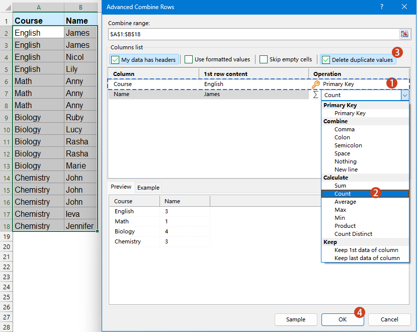
النتيجة: سيولّد Kutools جدولًا يحتوي على العدد الفريد استنادًا إلى العمود الذي حددته.
عدد القيم الفريدة في نطاق بناءً على عمود آخر باستخدام دالتي UNIQUE وFILTER
تقدم إصدارات Excel 365 وExcel 2021 والإصدارات الأحدث دوال مصفوفة ديناميكية قوية مثل UNIQUE وFILTER، التي تجعل عد القيم الفريدة في نطاق بناءً على عمود آخر أسهل من أي وقت مضى.
أدخل أو انقل الصيغة أدناه إلى خلية فارغة لوضع النتيجة، ثم اسحب الصيغة لأسفل لتعبئة الخلايا الأخرى، راجع لقطة الشاشة:
=IFERROR(ROWS(UNIQUE(FILTER($B$2:$B$18,$A$2:$A$18=D2))), 0)
- FILTER($B$2:$B$18, $A$2:$A$18=D2)يُرشّح القيم في العمود B حيث تطابق القيمة المقابلة في العمود A القيمة الموجودة في الخلية D2.
- UNIQUE(...): احذف التكرارات من القائمة المرشّحة، واحتفظ بالقيم الفريدة فقط.
- ROWS(...)تحسب عدد الصفوف في القائمة الفريدة، مما يُعطيك فعليًا عدد القيم الفريدة.
- IFERROR(..., 0)في حال حدوث خطأ (مثل عدم وجود قيم مطابقة في العمود A)، تُرجع الصيغة القيمة 0 بدلاً من عرض رسالة خطأ.
باختصار، يمكنك حساب عدد القيم الفريدة في نطاق بناءً على عمود آخر في Excel بعدة طرق، كلٌّ منها يناسب إصدارات مختلفة وتفضيلات المستخدمين. وبمجرد اختيارك الطريقة الأنسب لإصدار Excel الخاص بك وسير عملك، ستتمكن من إدارة بياناتك وتحليلها بكفاءة ودقة وسهولة. إذا كنت مهتمًا باستكشاف المزيد من نصائح وحيل Excel،فإن موقعنا يوفّر آلاف الدروس التعليمية.
مقالات ذات صلة:
كيف يمكنك حساب عدد القيم الفريدة في نطاق معين في Excel؟
كيف يمكن عد القيم الفريدة في نطاق ضمن عمود تم تطبيق التصفية عليه في Excel؟
كيف تحسب القيم المتماثلة أو المكررة مرة واحدة فقط في عمود؟
أفضل أدوات الإنتاجية لمكتبتك
عزِّز مهاراتك في Excel باستخدام Kutools لـ Excel، وعايش الكفاءة كما لم تفعل من قبل.يقدّم Kutools لـ Excel أكثر من 300 ميزة متقدمة لتعزيز الإنتاجية ووقت الحفظ.انقر هنا للحصول على الميزة التي تحتاجها أكثر من غيرها...
يجلب Office Tab واجهة ذات علامات تبويب إلى Office، ويجعل عملك أسهل بكثير
- تمكّن من التحرير والقراءة باستخدام علامات التبويب في Word وExcel وPowerPoint، وPublisher وAccess وVisio وProject.
- افتح وأنشئ مستندات متعددة في علامات تبويب جديدة داخل النافذة نفسها، بدلاً من فتح نوافذ جديدة.
- يزيد إنتاجيتك بنسبة 50% ويوفّر لك مئات نقرات الفأرة كل يوم!
جميع الإضافات من Kutools في برنامج تثبيت واحد!
Kutools for Office حزمةٌ تحتوي على إضافاتٍ مخصصة لتطبيقات Excel وWord وOutlook وPowerPoint، إلى جانب Office Tab Pro، مما يجعلها الخيار المثالي للفِرق التي تعمل عبر تطبيقات Office.
- حزمة شاملة واحدة— إضافات Excel وWord وOutlook وPowerPoint بالإضافة إلى Office Tab Pro
- برنامج تثبيت واحد، ترخيص واحد— الإعداد خلال دقائق (جاهز لـ MSI)
- يعمل بشكل أفضل معًا— إنتاجية ميسَّرة عبر تطبيقات Office
- تجربة مجانية لمدة 30 يومًا بكامل الميزات— بدون تسجيل، بدون بطاقة ائتمان
- أفضل قيمة— وفِّر مقارنةً بشراء الإضافات بشكل منفصل