كيف يمكن إخفاء جزءٍ فقط من قيمة الخلية في Excel؟

افترض أن لديك ورقة تحتوي على بعض المعلومات العامة عن الموظفين، لكن بعضها خاص مثل أرقام الضمان الاجتماعي. الآن تريد إخفاء جزء من هذه الأرقام كما هو موضح في لقطة الشاشة أدناه، فكيف يمكنك حل ذلك بسرعة؟

إخفاء أرقام الضمان الاجتماعي جزئيًا باستخدام تعيين تنسيق الخلية

إخفاء جزء من النص أو الرقم باستخدام الصيغ

إخفاء أرقام الضمان الاجتماعي جزئيًا باستخدام تعيين تنسيق الخلية

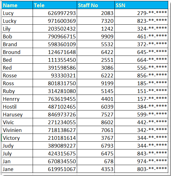
لإخفاء جزء من أرقام الضمان الاجتماعي في Excel، يمكنك تطبيق تنسيق خاص للخلايا لإنجاز هذه المهمة بسهولة.

1. حدد الأرقام التي تريد إخفاءها جزئيًا، ثم انقر بزر الماوس الأيمن واخترتعيين تنسيق الخليةمن القائمة السياقية. راجع لقطة الشاشة:

2. بعد ذلك، في مربع حوارتعيين تنسيق الخلية، انقر على علامة التبويبرقم، ثم اخترمخصصمن جزءالفئة، وأدخل التنسيق التالي000،«-**-****»في حقلالنوعالموجود في الجزء الأيمن. راجع لقطة الشاشة:

3. انقر علىموافق، وسيتم الآن إخفاء الأجزاء التي حددتها من الأرقام.

ملاحظة: سيتم تقريب الرقم لأعلى إذا كان الرقم الرابع أكبر من أو يساوي 5.

افتح سحر إكسل مع KUTOOLS AI

• التنفيذ الذكي: نفِّذ عمليات الخلايا، وحلِّل البيانات، وأنشئ المخططات البيانية — كل ذلك بأوامر بسيطة!
• الصيغ المخصصة: أنشئ صيغًا مخصصة لتبسيط سير عملك.
• برمجة VBA: اكتب وأَنفِذ أكواد VBA بسلاسة تامة.
• تفسير الصيغ: افهم الصيغ المعقدة بسهولة!
• ترجمة النصوص: اكسر الحواجز اللغوية في جداولك الإلكترونية!

حسِّن قدراتك في إكسل بأدوات مدعومة بالذكاء الاصطناعي.حمِّل الآنوجرِّب الكفاءة كما لم تفعل من قبل!

إخفاء جزء من النص أو الرقم باستخدام الصيغ

بالطريقة السابقة، يمكنك إخفاء جزءٍ من الأرقام فقط. أما إذا رغبت في إخفاء جزءٍ من الأرقام أو النصوص، فاتبع الخطوات التالية:

هنا سنقوم بإخفاء أول أربع أرقام من رقم جواز السفر.

اختر خلية فارغة بجانب رقم جواز السفر، مثل F22، وأدخل الصيغة التالية: =«****» & RIGHT(E22,5)، ثم اسحب مقبض التعبئة عبر الخلايا التي ترغب في تطبيق الصيغة عليها.

تلميح:

إذا كنت تريد إخفاء آخر أربعة أرقام، استخدم هذه الصيغة،= LEFT(H2,5)&«****»

إذا كنت تريد إخفاء الثلاثة أرقام الوسطى، استخدم هذه الصيغة=LEFT(H2,3)&«***»&RIGHT(H2,3)

أفضل أدوات الإنتاجية لمكتبتك

🤖	KUTOOLS AI مساعد: ثوّر تحليل البيانات استنادًا إلى:التنفيذ الذكي   |  إنشاء الكود|  إنشاء الصيغ المخصصة  |  تحليل البيانات وإنشاء المخططات البيانية|  استدعاء الوظائف المحسنة…
	الميزات الشائعة:البحث، التمييز أو وضع علامة على المكررات   |  حذف الصفوف الفارغة   |  دمج الأعمدة أو الخلايا دون فقدان البيانات   |  التقريب بدون استخدام الصيغة...
	بحث متقدم:VLookup متعدد المعايير  |  VLookup متعدد القيم  |   VLookup عبر أوراق متعددة   |   مطابقة غامضة....
	قائمة منسدلة متقدمة:إنشاء قائمة منسدلة بسرعة   |  قائمة منسدلة تابعة   |  قائمة منسدلة متعددة الاختيار....
	مدير الأعمدة:إضافة عدد محدد من الأعمدة|نقل الأعمدة|تبديل حالة ظهور الأعمدة المخفية|مقارنة النطاقات والأعمدة...
	ميزات مميزة:التركيز على الشبكة   |  عرض التصميم   |شريط الصيغ المحسن   | مدير الدفتر والورقة   |  مكتبة الموارد(نص تلقائي)|  أداة اختيار التاريخ   |  تجميع ورقات العمل  |  تشفير/فك تشفير الخلايا   | إرسال رسائل البريد الإلكتروني حسب القائمة   |  مرشح متقدم   |   تصفية خاصة(تصفية الخلايا التي تحتوي على خط عريض/مائل/يتوسطه خط...) ...
	أفضل 15 مجموعات الأدوات:12 أدواتالنصوص(إضافة نص،حذف الأحرف المحددة، ...)|   50+أنواعالمخططات البيانية(مخطط جانت، ...)|   40+ صيغعملية(حساب العمر بناءً على تاريخ الميلاد، ...)|   19 أدواتالإدراج(إدراج رمز QR،إدراج صورة من المسار، ...)|   12 أدواتالتحويل(تحويل إلى كلمات،تحويل العملة، ...)|   7 أدواتدمج وتقسيم(دمج متقدم للصفوف،تقسيم الخلايا، ...)|... وأكثر من ذلك

استخدم Kutools باللغة التي تفضلها – يدعم الإنجليزية والإسبانية والألمانية والفرنسية والصينية و40+ لغات أخرى!

عزِّز مهاراتك في Excel باستخدام Kutools لـ Excel، وعايش الكفاءة كما لم تفعل من قبل.يقدّم Kutools لـ Excel أكثر من 300 ميزة متقدمة لتعزيز الإنتاجية ووقت الحفظ.انقر هنا للحصول على الميزة التي تحتاجها أكثر من غيرها...

مزيد من التفاصيل حول Kutools لـ Excel...تنزيل مجاني...

---

يجلب Office Tab واجهة ذات علامات تبويب إلى Office، ويجعل عملك أسهل بكثير

• تمكّن من التحرير والقراءة باستخدام علامات التبويب في Word وExcel وPowerPoint، وPublisher وAccess وVisio وProject.
• افتح وأنشئ مستندات متعددة في علامات تبويب جديدة داخل النافذة نفسها، بدلاً من فتح نوافذ جديدة.
• يزيد إنتاجيتك بنسبة 50% ويوفّر لك مئات نقرات الفأرة كل يوم!

مزيد من التفاصيل حول Office Tab...تنزيل مجاني...

---

جميع الإضافات من Kutools في برنامج تثبيت واحد!

Kutools for Office حزمةٌ تحتوي على إضافاتٍ مخصصة لتطبيقات Excel وWord وOutlook وPowerPoint، إلى جانب Office Tab Pro، مما يجعلها الخيار المثالي للفِرق التي تعمل عبر تطبيقات Office.

• حزمة شاملة واحدة— إضافات Excel وWord وOutlook وPowerPoint بالإضافة إلى Office Tab Pro
• برنامج تثبيت واحد، ترخيص واحد— الإعداد خلال دقائق (جاهز لـ MSI)
• يعمل بشكل أفضل معًا— إنتاجية ميسَّرة عبر تطبيقات Office
• تجربة مجانية لمدة 30 يومًا بكامل الميزات— بدون تسجيل، بدون بطاقة ائتمان
• أفضل قيمة— وفِّر مقارنةً بشراء الإضافات بشكل منفصل

مزيد من التفاصيل حول Kutools for Office...تنزيل مجاني...