كيف يمكن تغيير لون الشكل في Excel بناءً على قيمة خلية معينة؟
قد يكون تغيير لون الشكل في Excel استنادًا إلى قيمة خلية معيّنة أمرًا مثيرًا للاهتمام! فعلى سبيل المثال، إذا كانت قيمة الخلية A1 أقل من 100، يصبح لون الشكل أحمر؛ وإذا كانت بين 100 و200، يتحول إلى الأصفر؛ وعند تجاوزها 200، يصبح أخضر — كما يظهر في لقطة الشاشة التالية. وفي هذا المقال، سنعرض لك طريقة تغيير لون الشكل تلقائيًا بناءً على قيمة الخلية!

تغيير لون الشكل استنادًا إلى قيمة الخلية باستخدام كود VBA
تغيير لون الشكل استنادًا إلى قيمة الخلية باستخدام كود VBA
يمكن أن يساعدك كود VBA أدناه في تغيير لون الشكل استنادًا إلى قيمة خلية، يُرجى اتباع الخطوات التالية:
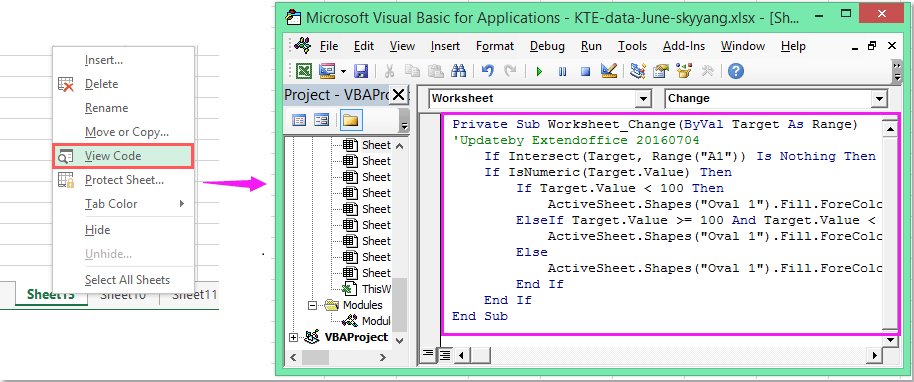
1. انقر بزر الماوس الأيمن على لسان التبويب الخاص بالورقة التي تريد تغيير لون خلفيتها، ثم اخترعرض الكود (View Code)من قائمة السياق. بعد فتح نافذةMicrosoft Visual Basic for Applications، يُرجى نسخ ولصق الكود التالي في نافذةالوحدة النمطية (Module)الفارغة.
كود VBA: تغيير لون الشكل استنادًا إلى قيمة الخلية:
Private Sub Worksheet_Change(ByVal Target As Range)
'Updateby Extendoffice 20160704
    If Intersect(Target, Range("A1")) Is Nothing Then Exit Sub
    If IsNumeric(Target.Value) Then
        If Target.Value < 100 Then
            ActiveSheet.Shapes("Oval 1").Fill.ForeColor.RGB = vbRed
        ElseIf Target.Value >= 100 And Target.Value < 200 Then
            ActiveSheet.Shapes("Oval 1").Fill.ForeColor.RGB = vbYellow
        Else
            ActiveSheet.Shapes("Oval 1").Fill.ForeColor.RGB = vbGreen
        End If
    End If
End Sub
2. بعد إدخال قيمة في الخلية A1، سيتغيّر لون الشكل وفقًا للقيمة التي عرّفتها.
ملاحظة: في الكود أعلاه،A1 هي الخلية التي سيتغيّر لون الشكل بناءً على قيمتها، وOval 1 هو اسم الشكل الذي أدرجته، ويمكنك تغييرهما حسب احتياجاتك.
أفضل أدوات الإنتاجية لمكتبتك
عزِّز مهاراتك في Excel باستخدام Kutools لـ Excel، وعايش الكفاءة كما لم تفعل من قبل.يقدّم Kutools لـ Excel أكثر من 300 ميزة متقدمة لتعزيز الإنتاجية ووقت الحفظ.انقر هنا للحصول على الميزة التي تحتاجها أكثر من غيرها...
يجلب Office Tab واجهة ذات علامات تبويب إلى Office، ويجعل عملك أسهل بكثير
- تمكّن من التحرير والقراءة باستخدام علامات التبويب في Word وExcel وPowerPoint، وPublisher وAccess وVisio وProject.
- افتح وأنشئ مستندات متعددة في علامات تبويب جديدة داخل النافذة نفسها، بدلاً من فتح نوافذ جديدة.
- يزيد إنتاجيتك بنسبة 50% ويوفّر لك مئات نقرات الفأرة كل يوم!
جميع الإضافات من Kutools في برنامج تثبيت واحد!
Kutools for Office حزمةٌ تحتوي على إضافاتٍ مخصصة لتطبيقات Excel وWord وOutlook وPowerPoint، إلى جانب Office Tab Pro، مما يجعلها الخيار المثالي للفِرق التي تعمل عبر تطبيقات Office.
- حزمة شاملة واحدة— إضافات Excel وWord وOutlook وPowerPoint بالإضافة إلى Office Tab Pro
- برنامج تثبيت واحد، ترخيص واحد— الإعداد خلال دقائق (جاهز لـ MSI)
- يعمل بشكل أفضل معًا— إنتاجية ميسَّرة عبر تطبيقات Office
- تجربة مجانية لمدة 30 يومًا بكامل الميزات— بدون تسجيل، بدون بطاقة ائتمان
- أفضل قيمة— وفِّر مقارنةً بشراء الإضافات بشكل منفصل