كيف يمكن عرض الاسم المقابل لأعلى درجة في Excel؟
عند تحليل الأداء أو النتائج في Excel، ستجد نفسك غالبًا بحاجة إلى تحديد الشخص الذي حقق أعلى درجة ضمن مجموعة بيانات تتضمّن أسماءً وقيمًا مرتبطة بها. فعلى سبيل المثال، قد يكون لديك أسماء الطلاب في عمودٍ واحد ودرجات اختباراتهم في عمودٍ آخر. والهدف هنا لا يقتصر على معرفة أعلى درجة فحسب، بل يمتد ليشمل عرض اسم (أو الأسماء، في حال وجود تعادل) للشخص الذي حقق أفضل نتيجة. ويُستخدم هذا النهج بشكل شائع في سيناريوهات مثل تتبع أفضل موظفي المبيعات، أو تقييم درجات الطلاب، أو نتائج تقييم الموظفين، أو أي سياقٍ تكون فيه التصنيفات ذات أهمية.
فيما يلي مجموعة من الحلول العملية، مرفقة بتعليمات خطوة بخطوة ونصائح فعّالة لمساعدتك على تجنب الأخطاء الشائعة. اختر الحل الأنسب لحجم بياناتك ومتطلبات إعداد التقارير لديك.
عرض الاسم المقابل لأعلى درجة باستخدام الصيغ
رمز VBA - العثور تلقائيًا على الاسم (الأسماء) لأعلى درجة وعرضه
جدول بيانات محوري - استخدام جدول بيانات محوري لعرض الاسم المقابل لأعلى درجة
عرض الاسم المقابل لأعلى درجة باستخدام الصيغ
لاسترجاع اسم الشخص الحاصل على أعلى درجة، تساعدك الصيغ التالية على تحقيق الناتج المطلوب بسهولة. وهي طريقة مثالية لمجموعات البيانات الصغيرة والمتوسطة، وتُعدّ حلاً سريعًا وفعالًا لتحديد أفضل أداء دون الحاجة إلى أدوات إضافية.
لإيجاد الاسم المرتبط بأعلى درجة، استخدم تركيبةINDEXوMATCHعلى النحو التالي:
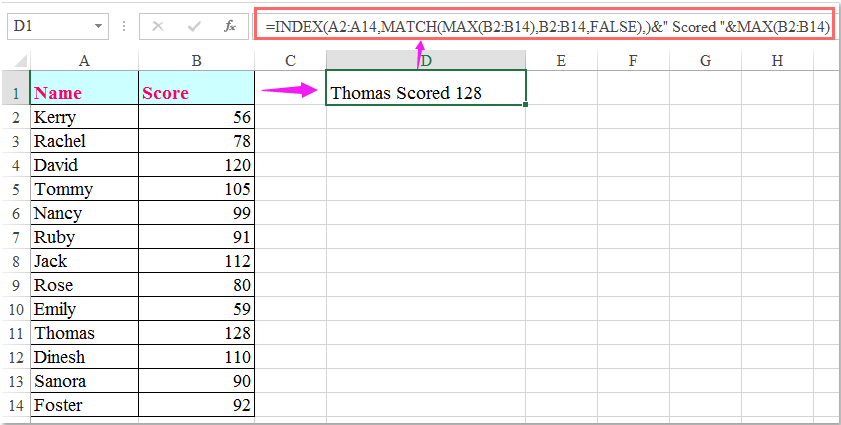
1. أدخل الصيغة التالية في خلية فارغة حيث تريد عرض الاسم (مثل الخلية C2):
=INDEX(A2:A14,MATCH(MAX(B2:B14),B2:B14,FALSE))&" Scored "&MAX(B2:B14)بعد كتابة الصيغة، اضغطEnter للتأكيد. ستُرجع الصيغة أول اسم تجده يحتوي على أعلى درجة. فعلى سبيل المثال، إذا حصل كلٌ من جون وأليس على 98، فستُرجع الصيغة الاسم الأول فقط.
ملاحظات:
1. في الصيغة أعلاه،A2:A14 هو نطاق الأسماء الذي تريد استخراج الاسم منه، وB2:B14 هو نطاق الدرجات. تأكد من أن النطاقات تتطابق تمامًا مع بياناتك.
2. تُرجع الصيغة أول اسم مطابق فقط. إذا كان هناك أكثر من شخص يشتركون في أعلى درجة، فقد ترغب في عرض جميع الأسماء؛ راجع الحل العملي أدناه.
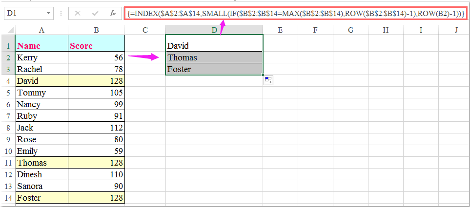
أدخل الصيغة التالية في أي خلية (مثل D2):
=INDEX($A$2:$A$14,SMALL(IF($B$2:$B$14=MAX($B$2:$B$14),ROW($B$2:$B$14)-1),ROW(B2)-1))بعد كتابة الصيغة، اضغطCtrl + Shift + Enter في نفس الوقت (وليس مفتاح Enter وحده) لتحويلها إلى صيغة صفيف. سيظهر الاسم الأول الحاصل على أعلى درجة. بعد ذلك، حدد خلية الصيغة واسحب مقبض التعبئة للأسفل حتى تبدأ قيم الخطأ بالظهور—حيث سيعرض كل صف اسمًا آخر من أولئك الذين يشاركون في المركز الأول. هذه الطريقة مفيدة جدًّا عندما تكون هناك درجات متعادلة وترغب في عرض جميع الفائزين!
إذا كانت نسختك من Excel تدعم المصفوفات الديناميكية (مثل Office 365 أو Excel 2021 والإصدارات الأحدث)، فيمكنك اعتماد نهج أكثر مباشرة. جرّب إدخال هذه الصيغة في خلية، ثم اضغط Enter ببساطة:
=FILTER(A2:A14,B2:B14=MAX(B2:B14))ستُخرِج هذه الصيغة تلقائيًا جميع الأسماء الأولى في الخلايا الموجودة أسفلها، دون الحاجة إلى السحب أو استخدام اختصارات لوحة المفاتيح الخاصة—وهي طريقة مريحة وفعّالة لإصدارات Excel الحديثة.
الصيغ قوية لإجراء استعلامات سريعة، لكنها قد لا تكون الخيار الأمثل لمجموعات البيانات الضخمة جدًّا، إذ قد يتأثر الأداء عند التعامل مع آلاف الصفوف. علاوةً على ذلك، تتطلب الصيغ مراجع نطاقات ثابتة لضمان دقة النتائج في حال إضافة صفوف أو حذفها—لذا تأكد دائمًا من اختيار بياناتك بعناية.
رمز VBA - العثور تلقائيًا على الاسم (الأسماء) لأعلى درجة وعرضه
يُعد استخدام ماكروهات VBA وسيلة مرنة وأوتوماتيكية للعثور على جميع الأسماء المرتبطة بأعلى درجة في مجموعة البيانات الخاصة بك وعرضها، خاصةً عندما تصبح الصيغ معقدة أو غير كافية للقوائم الكبيرة. ويمنحك VBA القدرة على تخصيص المنطق بما يتناسب تمامًا مع احتياجات تقريرك، كما يتعامل تلقائيًا مع التحديثات، مما يجعله خيارًا مثاليًا للتحليل المتكرر أو المعالجة الدفعية.
1. افتح مصنف Excel الخاص بك، ثم انقر فوقالمطور > Visual Basic. في نافذةMicrosoft Visual Basic for Applications، انقر فوقإدراج > وحدة نمطيةلإدراج وحدة نمطية فارغة.
انسخ ولصق رمز VBA التالي في نافذة الوحدة النمطية:
Sub ShowTopNames()
    Dim rngNames As Range, rngScores As Range, outCell As Range
    Dim nArr As Variant, sArr As Variant
    Dim i As Long, maxVal As Double, hasVal As Boolean
    Dim namesBuf As String
    On Error Resume Next
    Set rngNames = Application.InputBox("Please select the name column (single column)", "Top Names", Type:=8)
    Set rngScores = Application.InputBox("Please select the score column (single column, same rows as names)", "Top Names", Type:=8)
    Set outCell = Application.InputBox("Please select the output cell (optional, click Cancel to skip)", "Top Names", Type:=8)
    On Error GoTo 0
    If rngNames Is Nothing Or rngScores Is Nothing Then Exit Sub
    If rngNames.Rows.Count <> rngScores.Rows.Count Or rngNames.Columns.Count <> 1 Or rngScores.Columns.Count <> 1 Then
        MsgBox "Range mismatch: Name column and score column must be single columns with the same number of rows.", vbExclamation
        Exit Sub
    End If
    nArr = rngNames.Value2
    sArr = rngScores.Value2
    hasVal = False
    For i = 1 To UBound(sArr, 1)
        If IsNumeric(sArr(i, 1)) And Not IsEmpty(sArr(i, 1)) Then
            If Not hasVal Then
                maxVal = CDbl(sArr(i, 1))
                hasVal = True
            ElseIf CDbl(sArr(i, 1)) > maxVal Then
                maxVal = CDbl(sArr(i, 1))
            End If
        End If
    Next i
    If Not hasVal Then
        MsgBox "No valid numeric values found in the score column.", vbInformation
        Exit Sub
    End If
    rngNames.EntireRow.Interior.ColorIndex = xlNone
    For i = 1 To UBound(sArr, 1)
        If IsNumeric(sArr(i, 1)) Then
            If CDbl(sArr(i, 1)) = maxVal Then
                rngNames.Cells(i, 1).EntireRow.Interior.Color = RGB(255, 255, 153) ' Light yellow
                If Len(namesBuf) > 0 Then namesBuf = namesBuf & ", "
                namesBuf = namesBuf & CStr(nArr(i, 1))
            End If
        End If
    Next i
    If Not outCell Is Nothing Then
        outCell.Value = "Top Score: " & maxVal & " | Name(s): " & namesBuf
    End If
    MsgBox "Top Score = " & maxVal & vbCrLf & "Name(s): " & namesBuf, vbInformation, "Highest Score"
End Sub
2. بعد ذلك، اضغط على مفتاحF5 لتشغيل هذا الرمز. ستظهر لك ثلاث نوافذ منبثقة: حدد عمود الأسماء (عمود واحد). اسحب لتحديد الأسماء فقط (مثل A2:A14) → موافق. حدد عمود الدرجات (عمود واحد، نفس الصفوف الخاصة بالأسماء). اسحب لتحديد الدرجات (مثل B2:B14) → موافق. حدد خلية الإخراج (اختياري). انقر فوق خلية وجهة (مثل D2) لوضع النتيجة.
بعد تشغيل الرمز، ستظهر النتيجة في الخلية المحددة، ويتم تمييز الصف بأكمله—بما في ذلك جميع الطلاب الحاصلين على الدرجة العليا—باللون الأصفر الفاتح.
جدول بيانات محوري - استخدام جدول بيانات محوري لعرض الاسم المقابل لأعلى درجة
توفر جدول بيانات محوري في Excel طريقة مرئية وتفاعلية لتحليل البيانات وتلخيصها. وهي مفيدة بشكل خاص للتعامل مع مجموعات البيانات الكبيرة، وإجراء تحليل مجمّع، وتحديد القيمة القصوى بسرعة، مثل تحديد أفضل مُنجز في كل فئة أو بشكل عام في القائمة. ولا تتطلب هذه الطريقة صيغًا أو برمجة، مما يجعلها مناسبة للمستخدمين الذين يفضلون الحلول التي تعتمد على النقر والمؤشر والمهمات التقريرية المنتظمة.
سير العمل الأساسي لاستخدام جدول بيانات محوري لهذا الغرض هو كما يلي:
1. حدد أي خلية داخل نطاق البيانات الخاص بك (الذي يشمل عمودَي الأسماء والدرجات)، ثم انتقل إلىإدراج > جدول محوري. في مربع الحوار، تأكد من صحة نطاق البيانات، واختر وضع الجدول المحوري في ورقة جديدة أو ورقة عمل موجودة حسب تفضيلك.
2. في لوحة حقول الجدول المحوري، اسحب حقلالاسمإلى منطقةالصفوف، واسحب حقلالدرجةإلى منطقةالقيم. سيتم ضبط منطقة القيم افتراضيًا على «المجموع» أو «العدد». انقر على السهم المنسدل لحقلالدرجةفي منطقة القيم، وحددقيمة إعدادات الحقول، ثم اخترالحد الأقصىكدالة التلخيص، وانقر علىموافق.
3. الآن يعرض جدول البيانات المحوري أعلى درجة لكل اسم. ولإبراز أفضل مُنجز على الإطلاق، رتّب عمود «الحد الأقصى للدرجة» ترتيبًا تنازليًّا—سيكون الاسم في الأعلى هو صاحب أعلى درجة (أو أحد المتعادلين على المركز الأول). كما يمكنك تطبيق عوامل التصفية أو استخدام التنسيق الشرطي للتأكيد البصري.
إذا كنت تريد عرضفقطأفضل مُنجز (أو المُنجزين)، فطابِق عوامل تصفية القيم: انقر على السهم المنسدل في تسميات الصفوف الخاصة بالأسماء، وحددتصفية القيم >يساوي، ثم اضبط القيمة على أعلى درجة (ويمكنك تحديدها مؤقتًا بفرز القيم أو بالتحقق من أعلى رقم في عمود الحد الأقصى للدرجة). بهذه الطريقة، يُمكنك التركيز في التقرير على اسم (أو أسماء) الفائزين فقط.
يتميّز الجدول المحوري بقوته الاستكشافية: يمكنك بسهولة تحديث بياناتك أو توسيعها أو تصفيتها، وسيقوم الجدول المحوري تلقائيًا بإعادة حساب النتائج فور التحديث. ومع ذلك، إذا كانت مجموعة البيانات الخاصة بك تتغيّر باستمرار، فاحرص دائمًا على النقر بزر الماوس الأيمن على جدولك المحوري واختيارتحديثبعد إضافة بيانات جديدة.
قد يتطلب الجدول المحوري إعدادًا أوليًا بسيطًا، لكنه يوفّر إعداد تقارير مرنة ومقارنات عبر المجموعات—مثلًا حسب القسم أو الفريق—إذا كانت بياناتك تحتوي على فئات إضافية.
إذا واجهت مشكلات في التلخيص أو الفرز، فتحقق من أن بياناتك لا تحتوي على خلايا فارغة وأن اسم الشرط مكتوبة بشكل متسق. وعند استخدام قوائم كبيرة، فإن الانتباه الدقيق إلى نطاق المصدر يضمن أن جدول بيانات محوري يأخذ في الاعتبار جميع البيانات ذات الصلة.

افتح سحر إكسل مع KUTOOLS AI
- التنفيذ الذكي: نفِّذ عمليات الخلايا، وحلِّل البيانات، وأنشئ المخططات البيانية — كل ذلك بأوامر بسيطة!
- الصيغ المخصصة: أنشئ صيغًا مخصصة لتبسيط سير عملك.
- برمجة VBA: اكتب وأَنفِذ أكواد VBA بسلاسة تامة.
- تفسير الصيغ: افهم الصيغ المعقدة بسهولة!
- ترجمة النصوص: اكسر الحواجز اللغوية في جداولك الإلكترونية!
أفضل أدوات الإنتاجية لمكتبتك
عزِّز مهاراتك في Excel باستخدام Kutools لـ Excel، وعايش الكفاءة كما لم تفعل من قبل.يقدّم Kutools لـ Excel أكثر من 300 ميزة متقدمة لتعزيز الإنتاجية ووقت الحفظ.انقر هنا للحصول على الميزة التي تحتاجها أكثر من غيرها...
يجلب Office Tab واجهة ذات علامات تبويب إلى Office، ويجعل عملك أسهل بكثير
- تمكّن من التحرير والقراءة باستخدام علامات التبويب في Word وExcel وPowerPoint، وPublisher وAccess وVisio وProject.
- افتح وأنشئ مستندات متعددة في علامات تبويب جديدة داخل النافذة نفسها، بدلاً من فتح نوافذ جديدة.
- يزيد إنتاجيتك بنسبة 50% ويوفّر لك مئات نقرات الفأرة كل يوم!
جميع الإضافات من Kutools في برنامج تثبيت واحد!
Kutools for Office حزمةٌ تحتوي على إضافاتٍ مخصصة لتطبيقات Excel وWord وOutlook وPowerPoint، إلى جانب Office Tab Pro، مما يجعلها الخيار المثالي للفِرق التي تعمل عبر تطبيقات Office.
- حزمة شاملة واحدة— إضافات Excel وWord وOutlook وPowerPoint بالإضافة إلى Office Tab Pro
- برنامج تثبيت واحد، ترخيص واحد— الإعداد خلال دقائق (جاهز لـ MSI)
- يعمل بشكل أفضل معًا— إنتاجية ميسَّرة عبر تطبيقات Office
- تجربة مجانية لمدة 30 يومًا بكامل الميزات— بدون تسجيل، بدون بطاقة ائتمان
- أفضل قيمة— وفِّر مقارنةً بشراء الإضافات بشكل منفصل