كيف تُظهر العنصر الأول في القائمة المنسدلة بدلاً من تركها فارغة؟
تُعد القائمة المنسدلة في أوراق عمل Excel ميزة عملية تُبسّط إدخال البيانات وتضمن اتساقه، إذ يكفي المستخدم أن يختار من بين خيارات معرّفة مسبقًا بدلًا من كتابة القيم يدويًّا. لكن قد تواجه أحيانًا موقفًا يكون فيه الخيار الأول عند النقر على خلية القائمة المنسدلة فارغًا، بدلًا من عرض أول عنصر بيانات فعلي. وغالبًا ما ينشأ هذا المشكل عندما تُعدَّل قائمة البيانات الأصلية وتبقى خلايا صفوف فارغة في نهايتها، أو عند حذف عناصر قريبة من النهاية، مما يؤدي إلى تضمين خلايا فارغة غير مقصودة في التحقق من صحة البيانات، لتظهر في أعلى القائمة. وخصوصًا مع القوائم الطويلة، فإن الحاجة الدائمة للتمرير عبر هذه الإدخالات الفارغة للوصول إلى أول عنصر صالح قد تكون غير فعّالة ومُحبِطة.

لا يُحسّن معالجة هذا الأمر تجربة المستخدم فحسب، بل يساعد أيضًا في تجنّب اختيار قيم فارغة عن طريق الخطأ، والتي قد تؤثر سلبًا على مهام معالجة البيانات أو إعداد التقارير اللاحقة. في هذه المقالة، ستتعرّف على طرق عملية لضمان ظهور أول إدخال في القائمة المنسدلة دائمًا في الأعلى، وبالتالي التخلّص من تلك الخانات الفارغة غير الضرورية.
إظهار العنصر الأول في القائمة المنسدلة تلقائيًّا بدلاً من الفراغ باستخدام كود VBA
استخدام جدول Excel كـ نطاق المصدر
إظهار العنصر الأول في القائمة المنسدلة بدلاً من الفراغ باستخدام وظيفة التحقق من الصلاحية (Data Validation)
إحدى الطرق الفعّالة لتجنب ظهور إدخالات فارغة في أعلى القائمة المنسدلة هي إعداد التحقق من الصلاحية باستخدام صيغة تُحدّد النطاق الصحيح ديناميكيًّا. ويضمن هذا الأسلوب تضمين الخلايا المملوءة فقط من قائمة المصدر، بغض النظر عن وجود أي صفوف فارغة ناتجة عن حذف البيانات في نهايتها. ويُعدّ هذا الحل مثاليًا خصوصًا للمستخدمين الذين يُعدّلون قائمة المصدر بشكل متكرر أو يفضلون إجراء تعديلات مباشرة قائمة على الصيغ دون الحاجة إلى استخدام ماكرو.
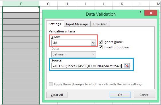
1. حدد الخلايا التي ترغب في إنشاء قائمة منسدلة فيها، ثم انتقل إلى شريط Excel وانقر علىبيانات > التحقق من الصلاحية > التحقق من الصلاحية. سيظهر مربع حوار التحقق من الصلاحية كما هو موضح أدناه:

2. ضمن علامة التبويبالإعداداتفي مربع حوار التحقق من الصلاحية، اضبط خيارالسماح بـعلىقائمة. وفي مربعالمصدر، أدخل هذه الصيغة للإشارة ديناميكيًّا فقط إلى النطاق الذي يحتوي على بيانات فعلية:
=OFFSET(Sheet3!$A$1,0,0,COUNTA(Sheet3!$A:$A)-1,1)
ملاحظة:في هذه الصيغة، يشيرSheet3 إلى الورقة التي تحتوي على بياناتك الأصلية، ويشيرA1 إلى الخلية الأولى في قائمتك. قم بتعديل هذه القيم حسب احتياجاتك لتتناسب مع تخطيط ورقة العمل الخاصة بك. ويضمن استخدام الدالة COUNTA تضمين الخلايا غير الفارغة فقط، بدءًا من الخلية A1. إذا كانت قائمة المصدر تحتوي على صفوف فارغة متعمَّدة داخلها (وليس فقط في نهايتها)، فقد لا تستبعد هذه الطريقة تلك الصفوف تمامًا، لذا تأكد من أن تكون قائمة المصدر متصلة دون فراغات لتحقيق أفضل النتائج.
3. انقر علىموافقلتطبيق الإعدادات. الآن، عند النقر على أيٍّ من خلايا القائمة المنسدلة التي قمت بتكوينها، ستعرض القائمة أول عنصر بيانات فعلي في الأعلى. وسيظل هذا صحيحًا حتى لو تغيّرت البيانات الأصلية، طالما أن النطاق يغطي جميع العناصر في العمود A ولم توجد خلايا فارغة داخل الكتلة الرئيسية من البيانات. راجع النتيجة أدناه:

تلميح:إذا احتجت لاحقًا إلى توسيع قائمة المصدر أو تقليصها، فلن تحتاج إلى تحديث إعدادات التحقق من الصلاحية — فالصيغة ستُعدِّل نفسها تلقائيًّا، بشرط ألا تحتوي بداية النطاق على خلايا فارغة. ومع ذلك، ضع في اعتبارك أنه إذا وُجدت خلية فارغة داخل القائمة (وليس فقط في نهايتها)، فسيتم تخطيها عند حساب العدد، وقد تؤدي إلى ظهور فراغات غير مقصودة في القائمة المنسدلة.
مشكلة محتملة:إذا كان نطاق المصدر الخاص بك يحتوي على فراغات متعمدة، أو يحتوي على خلايا مدمجة أو بيانات غير متصلة، ففكّر في استخدام جدول Excel كنطاق مصدرك، أو راجع طريقة VBA أدناه للتعامل معها بمرونة أكبر.
إظهار العنصر الأول في القائمة المنسدلة تلقائيًّا بدلاً من الفراغ باستخدام كود VBA
في بعض السيناريوهات، قد لا يكفي تعديل مصدر التحقق من الصلاحية وحده—مثلًا، إذا كانت بياناتك تتغيّر باستمرار، أو إذا وُجد خطر ظهور خلايا فارغة لأسباب هيكلية ضمن نطاق المصدر. باستخدام كود VBA بسيط، يمكنك ضمان عرض القائمة المنسدلة واختيار أول عنصر متاح تلقائيًّا كلما تم تنشيط خلية تحتوي على تحقق من الصلاحية. ويُسهم ذلك أيضًا في تسريع إدخال البيانات، إذ يقلل عدد النقرات التي يحتاجها المستخدم.
1. بعد إدراج قائمة منسدلة، انقر بزر الماوس الأيمن على تبويب الورقة التي تحتوي على القائمة المنسدلة، ثم اخترعرض الكودمن قائمة السياق. سيُفتح محررمايكروسوفت فيجوال بيسيك للتطبيقات (Microsoft Visual Basic for Applications). في النافذة التي تظهر، الصق الكود التالي في وحدة الورقة ذات الصلة (وليس في وحدة قياسية). وسيعمل هذا الكود في الخلفية لإعادة ضبط القائمة المنسدلة تلقائيًا في كل مرة تُحدِّد خليةً تحتوي على التحقق من الصلاحية:
كود VBA: إظهار أول عنصر بيانات في القائمة المنسدلة تلقائيًّا:
Private Sub Worksheet_SelectionChange(ByVal Target As Range)
'Updateby Extendoffice 20160725
    Dim xFormula As String
    On Error GoTo Out:
    xFormula = Target.Cells(1).Validation.Formula1
    If Left(xFormula, 1) = "=" Then
        Target.Cells(1) = Range(Mid(xFormula, 1)).Cells(1).Value
    End If
Out:
End Sub

2. بعد لصق الكود، احفظ ملفك (يفضّل كملف يدعم الماكرو بامتداد .xlsm)، ثم أغلق نافذة محرر VBA. الآن، عُد إلى ورقتك وجرب النقر على أي خلية تحتوي على قائمة منسدلة—فبمجرد تنشيط الخلية، سيظهر أول إدخال في قائمتك المنسدلة تلقائيًّا.
نصائح واعتبارات:يُعدّ هذا النهج باستخدام VBA مثاليًّا لتجربة مستخدم سلسة، خصوصًا مع القوائم المصدر الديناميكية أو الطويلة، أو تلك التي قد تحتوي على إدخالات فارغة لا يمكن تجنّبها. تذكّر تمكين الماكرو ليعمل الحل بشكل صحيح، وأبلغ المستخدمين الآخرين بهذا الملف، إذ إن بعض البيئات تقيّد استخدام الماكرو لأسباب أمنية.
استكشاف الأخطاء وإصلاحها:إذا بدا أن الكود لا يعمل، فتأكد أولًا من وضعه في نافذة كود الورقة الصحيحة في محرر VBA، وتأكد أيضًا من أن القائمة المنسدلة تعتمد على قائمة تحقق من الصلاحية قياسية.
قيد:لن يتم تشغيل حل VBA إلا إذا قام المستخدم بتحديد خلية تحتوي على قائمة منسدلة؛ إذ لا يعمل الحل إذا تم ملء الخلية بأي وسيلة أخرى (مثل نتائج الصيغ أو عبر اللصق). كما أنك إذا أزلت القائمة المنسدلة من الخلية، أو نقلتها إلى ورقة أخرى لا يحتوي كود VBA الخاص بها، فستفقد سلوك الاختيار التلقائي.
استخدام جدول Excel كـ نطاق المصدر
إذا كانت قائمة مصدر القائمة المنسدلة ديناميكية وترغب في صيانة أكثر سهولة، ففكّر في تحويل قائمة المصدر إلى جدول Excel. فالجداول تُعدّل حجمها تلقائيًّا عند إضافة البيانات أو حذفها، مما يضمن بقاء قائمتك مُحدَّثة دائمًا. ومع ذلك، ضع في اعتبارك أن جدول Excel لا يستبعد الخلايا الفارغة تلقائيًّا—فأي إدخالات فارغة داخل الجدول ستظل تظهر في القائمة المنسدلة ما لم تقم بفلترتها صراحةً (مثلًا، باستخدام دالة FILTER المتاحة في Excel 365 وExcel 2021).
1. حدد بياناتك الأصلية، ثم اضغط علىCtrl + T لتحويلها إلى جدول. تأكد من خلو الصف العلوي من الخلايا الفارغة، وعيّن للجدول اسمًا ذا معنى—مثلMyList—باستخدام علامة تبويب «تصميم الجدول».
2. عند إعداد التحقق من الصلاحية، استخدم المرجع المنظّم لعمود جدولك. في مربّعالمصدرفي التحقق من الصلاحية، اكتب:
=INDIRECT("MyList[Column1]")استبدلColumn1 باسم العمود الفعلي (عنوان العمود). بهذه الطريقة، يتم تضمين جميع العناصر المملوءة في عمود الجدول ديناميكيًّا، مع الحفاظ على سلامة القائمة أثناء تحديث البيانات.
يُعدّ هذا النهج مثاليًا بشكل خاص للبيئات التي تُحدَّث فيها البيانات الأصلية بانتظام، ويحتاج فيها عدة مستخدمين إلى إدارة القائمة المحققة بكفاءة.
أفضل أدوات الإنتاجية لمكتبتك
عزِّز مهاراتك في Excel باستخدام Kutools لـ Excel، وعايش الكفاءة كما لم تفعل من قبل.يقدّم Kutools لـ Excel أكثر من 300 ميزة متقدمة لتعزيز الإنتاجية ووقت الحفظ.انقر هنا للحصول على الميزة التي تحتاجها أكثر من غيرها...
يجلب Office Tab واجهة ذات علامات تبويب إلى Office، ويجعل عملك أسهل بكثير
- تمكّن من التحرير والقراءة باستخدام علامات التبويب في Word وExcel وPowerPoint، وPublisher وAccess وVisio وProject.
- افتح وأنشئ مستندات متعددة في علامات تبويب جديدة داخل النافذة نفسها، بدلاً من فتح نوافذ جديدة.
- يزيد إنتاجيتك بنسبة 50% ويوفّر لك مئات نقرات الفأرة كل يوم!
جميع الإضافات من Kutools في برنامج تثبيت واحد!
Kutools for Office حزمةٌ تحتوي على إضافاتٍ مخصصة لتطبيقات Excel وWord وOutlook وPowerPoint، إلى جانب Office Tab Pro، مما يجعلها الخيار المثالي للفِرق التي تعمل عبر تطبيقات Office.
- حزمة شاملة واحدة— إضافات Excel وWord وOutlook وPowerPoint بالإضافة إلى Office Tab Pro
- برنامج تثبيت واحد، ترخيص واحد— الإعداد خلال دقائق (جاهز لـ MSI)
- يعمل بشكل أفضل معًا— إنتاجية ميسَّرة عبر تطبيقات Office
- تجربة مجانية لمدة 30 يومًا بكامل الميزات— بدون تسجيل، بدون بطاقة ائتمان
- أفضل قيمة— وفِّر مقارنةً بشراء الإضافات بشكل منفصل