كيف يمكنني البحث عن أول قيمة غير صفرية في Excel وإرجاع رأس العمود المقابل لها؟
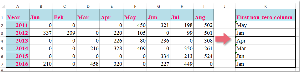
عند العمل مع البيانات في Excel، غالبًا ما تحتاج إلى تحديد موقع أول إدخال غير صفري في صفٍ ما، ثم عرض رأس العمود المرتبط به. فعلى سبيل المثال، إذا كانت كل صفوف مجموعة البيانات تمثّل عنصرًا أو شخصًا مختلفًا، بينما تمثّل الأعمدة فترات زمنية أو فئات، فقد ترغب في معرفة متى تظهر أول قيمة غير صفرية في كل صف. والتحقق يدويًّا من كل صف للعثور على هذه القيمة قد يستغرق وقتًا طويلاً، خاصة مع تزايد حجم البيانات. وأتمتة هذه العملية لا تحسّن الكفاءة فحسب، بل تقلّل أيضًا من الأخطاء، مما يجعل تحليلاتك أكثر موثوقية. ويعرض هذا المقال عدة طرق عملية لتحقيق هذا الهدف، بدءًا من استخدام صيغ Excel متعددة الاستخدامات، ووصولًا إلى توظيف ماكروهات VBA التي تُعدّ مفيدة بشكل خاص عند التعامل مع مجموعات بيانات ضخمة أو إعداد تقارير متكررة.
- البحث عن أول قيمة غير صفرية وإرجاع رأس العمود المقابل باستخدام صيغة
- استخدام ماكرو VBA للعثور على رأس العمود لأول قيمة غير صفرية في كل صف وإرجاعه
 البحث عن أول قيمة غير صفرية وإرجاع رأس العمود المقابل باستخدام صيغة
لتحديد رأس العمود في الصف الذي تظهر فيه أول قيمة غير صفرية بكفاءة، يمكنك استخدام صيغة مضمنة في Excel. ويُعدّ هذا النهج مثاليًا خصوصًا لمجموعات البيانات الصغيرة إلى المتوسطة الحجم، حيث تكون سهولة الإعداد وإعادة الحساب الفوري من الأولويات المهمة.
1. حدد خلية فارغة لعرض النتيجة؛ في هذا المثال، تم استخدام الخليةK2.
=INDEX($B$1:$I$1,MATCH(TRUE,INDEX(B2:I2<>0,),0))2. بعد إدخال الصيغة، اضغط علىEnter للتأكيد. بعد ذلك، حدد الخليةK2 واستخدم مقبض التعبئة لسحب الصيغة لأسفل وتطبيقها على بقية الصفوف حسب الحاجة.
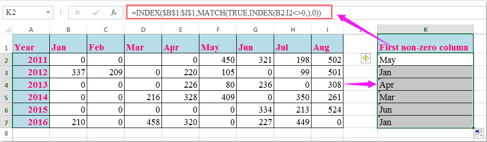
ملاحظة: في الصيغة أعلاه، يشيرB1:I1 إلى نطاق رؤوس الأعمدة التي ترغب في إرجاعها، بينما يمثلB2:I2 بيانات الصف الذي تقوم بتحليله للعثور على أول قيمة غير صفرية.
إذا كانت بياناتك تبدأ في أعمدة أو صفوف مختلفة، فلا تنسَ تعديل نطاقات الصيغة وفقًا لذلك. تعمل هذه الصيغة بكفاءة طالما أن هناك قيمة واحدة على الأقل غير صفرية في كل صف يتم تحليله؛ أما إذا كانت جميع القيم صفرًا، فستُرجع الصيغة خطأً. وفي مثل هذه الحالات، يُفضّل تضمين الصيغة داخل دالةIFERROR على النحو التالي:=IFERROR(INDEX($B$1:$I$1,MATCH(TRUE,INDEX(B2:I2<>0,),0)),"No non-zero") لإرجاع رسالة مخصصة بدلًا من الخطأ.
يُعد هذا الحل الصيغوي مثاليًّا عندما ترغب في نتائج ديناميكية تتجدَّد فورًا مع أي تغيير في بيانات الإدخال. ومع ذلك، عند التعامل مع مجموعات بيانات ضخمة جدًّا، قد تتأثر سرعة الحساب، وقد تفضِّل اعتماد نهج VBA لتحسين أتمتة سير العمل أو تقليل الاعتماد على العمليات اليدوية.
استخدام ماكرو VBA للعثور على رأس العمود لأول قيمة غير صفرية في كل صف وإرجاعه
إذا كنت غالبًا ما تحتاج إلى تنفيذ مهمة البحث هذه عبر العديد من الصفوف أو على مجموعات بيانات كبيرة، أو إذا رغبت في أتمتة العملية لتعزيز الكفاءة، فإن استخدام ماكرو VBA يُعد خيارًا عمليًّا للغاية. وتبرز فائدة هذه الطريقة بشكل خاص عند إنشاء تقارير دورية أو التعامل مع جداول بيانات تتغير أحجامها باستمرار، حيث يقوم الماكرو بالبحث في كل صف محدد عن أول قيمة غير صفرية، ثم يُرجع رأس العمود المقابل إلى الخلية المستهدفة.
1. انقر على تبويبالمطور > Visual Basic لفتح نافذةMicrosoft Visual Basic for Applications. (إذا لم يكن تبويب المطور ظاهرًا، يمكنك إضافته عبر)ملف > خيارات > تخصيص الشريط.) في محرر VBA، انقر علىإدراج > وحدة نمطية.
2.انسخ والصق كود VBA التالي في الوحدة النمطية الجديدة:
Sub LookupFirstNonZeroAndReturnHeader()
    Dim ws As Worksheet
    Dim dataRange As Range
    Dim headerRange As Range
    Dim outputCell As Range
    Dim r As Range
    Dim c As Range
    Dim firstNonZeroCol As Integer
    Dim i As Long
    Dim xTitleId As String
    On Error Resume Next
    xTitleId = "KutoolsforExcel"
    Set ws = Application.ActiveSheet
    Set dataRange = Application.InputBox("Select the data range (excluding headers):", xTitleId, Selection.Address, Type:=8)
    If dataRange Is Nothing Then Exit Sub
    Set headerRange = ws.Range(dataRange.Offset(-1, 0).Resize(1, dataRange.Columns.Count).Address)
    For i = 1 To dataRange.Rows.Count
        Set r = dataRange.Rows(i)
        firstNonZeroCol = 0

        For Each c In r.Columns
            If c.Value <> 0 And c.Value <> "" Then
                firstNonZeroCol = c.Column - dataRange.Columns(1).Column + 1
                Exit For
            End If
        Next c

        Set outputCell = r.Cells(1, r.Columns.Count + 1)

        If firstNonZeroCol > 0 Then
            outputCell.Value = headerRange.Cells(1, firstNonZeroCol).Value
        Else
            outputCell.Value = "No non-zero"
        End If
    Next i

    On Error GoTo 0
    MsgBox "Completed! Results are in the column to the right of your data.", vbInformation, "KutoolsforExcel"
End Sub
3. لتشغيل الماكرو، انقر على زرتشغيلأو اضغط على مفتاحF5. بعد ذلك، سيظهر لك مربع حوار يطلب منك تحديد نطاق البيانات (باستثناء رؤوس الأعمدة). وبعد تنفيذ الماكرو، سيتم ملء العمود الموجود فورًا على يمين نطاق البيانات المحدد برأس العمود لأول قيمة غير صفرية في كل صف، أو برسالة «لا توجد قيمة غير صفرية» إذا لم يتم العثور على أي قيمة غير صفرية.
يتميّز نهج VBA هذا بكفاءته الفائقة في تنفيذ المهام المتكررة، وهو مثالي للتعامل مع مجموعات البيانات الكبيرة، مما يقلل الجهد اليدوي بشكل كبير. ومع ذلك، تأكد من تفعيل الماكروات في بيئة Excel الخاصة بك، واحفظ دائمًا نسخة احتياطية من ملفك قبل تشغيل أي كود.
ملاحظة: إذا واجهت أخطاءً، فتأكد من أن تحديـدك يستثني صف الرؤوس ويتضمّن فقط صفوف البيانات.

افتح سحر إكسل مع KUTOOLS AI
- التنفيذ الذكي: نفِّذ عمليات الخلايا، وحلِّل البيانات، وأنشئ المخططات البيانية — كل ذلك بأوامر بسيطة!
- الصيغ المخصصة: أنشئ صيغًا مخصصة لتبسيط سير عملك.
- برمجة VBA: اكتب وأَنفِذ أكواد VBA بسلاسة تامة.
- تفسير الصيغ: افهم الصيغ المعقدة بسهولة!
- ترجمة النصوص: اكسر الحواجز اللغوية في جداولك الإلكترونية!
أفضل أدوات الإنتاجية لمكتبتك
عزِّز مهاراتك في Excel باستخدام Kutools لـ Excel، وعايش الكفاءة كما لم تفعل من قبل.يقدّم Kutools لـ Excel أكثر من 300 ميزة متقدمة لتعزيز الإنتاجية ووقت الحفظ.انقر هنا للحصول على الميزة التي تحتاجها أكثر من غيرها...
يجلب Office Tab واجهة ذات علامات تبويب إلى Office، ويجعل عملك أسهل بكثير
- تمكّن من التحرير والقراءة باستخدام علامات التبويب في Word وExcel وPowerPoint، وPublisher وAccess وVisio وProject.
- افتح وأنشئ مستندات متعددة في علامات تبويب جديدة داخل النافذة نفسها، بدلاً من فتح نوافذ جديدة.
- يزيد إنتاجيتك بنسبة 50% ويوفّر لك مئات نقرات الفأرة كل يوم!
جميع الإضافات من Kutools في برنامج تثبيت واحد!
Kutools for Office حزمةٌ تحتوي على إضافاتٍ مخصصة لتطبيقات Excel وWord وOutlook وPowerPoint، إلى جانب Office Tab Pro، مما يجعلها الخيار المثالي للفِرق التي تعمل عبر تطبيقات Office.
- حزمة شاملة واحدة— إضافات Excel وWord وOutlook وPowerPoint بالإضافة إلى Office Tab Pro
- برنامج تثبيت واحد، ترخيص واحد— الإعداد خلال دقائق (جاهز لـ MSI)
- يعمل بشكل أفضل معًا— إنتاجية ميسَّرة عبر تطبيقات Office
- تجربة مجانية لمدة 30 يومًا بكامل الميزات— بدون تسجيل، بدون بطاقة ائتمان
- أفضل قيمة— وفِّر مقارنةً بشراء الإضافات بشكل منفصل