كيف تجد الخلية غير الفارغة ذات الترتيب N في إكسل؟
كيف يمكنك العثور على القيمة الموجودة في الخلية غير الفارغة ذات الترتيب n ضمن عمود أو صف في إكسل وإرجاعها؟ في هذه المقالة، سأعرض لك بعض الصيغ المفيدة التي تساعدك على إنجاز هذه المهمة بسلاسة.
العثور على القيمة الموجودة في الخلية غير الفارغة ذات الترتيب n من عمود باستخدام صيغة
العثور على القيمة الموجودة في الخلية غير الفارغة ذات الترتيب n من صف باستخدام صيغة
 العثور على القيمة الموجودة في الخلية غير الفارغة ذات الترتيب n من عمود باستخدام صيغة
على سبيل المثال، لدي عمود من البيانات كما هو موضح في لقطة الشاشة التالية، وسأحصل الآن على القيمة الموجودة في ثالث خلية غير فارغة ضمن هذه القائمة.
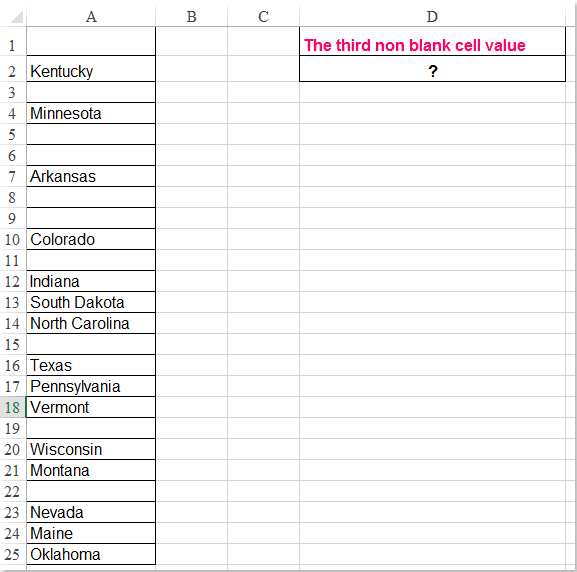
يرجى إدخال هذه الصيغة:=INDEX($A$1:$A$25,SMALL(ROW($A$1:$A$25)+(100*($A$1:$A$25=«»)), 3))&""في خلية فارغة حيث تريد عرض النتيجة، مثل D2، ثم اضغط على مفاتيحCtrl + Shift + Enterمعًا للحصول على النتيجة الصحيحة، انظر لقطة الشاشة:

ملاحظة: في الصيغة أعلاه،A1:A25 هي نطاق البيانات الذي تريد استخدامه، والرقم3 يشير إلى القيمة الموجودة في ثالث خلية غير فارغة تريد إرجاعها. إذا كنت ترغب في الحصول على ثاني خلية غير فارغة، فما عليك سوى تغيير الرقم 3 إلى 2 حسب الحاجة.
العثور على القيمة الموجودة في الخلية غير الفارغة ذات الترتيب n من صف باستخدام صيغة
إذا كنت تريد العثور على القيمة الموجودة في الخلية غير الفارغة ذات الترتيب n في صف وإرجاعها، فقد تساعدك الصيغة التالية، يرجى اتباع الخطوات التالية:
أدخل هذه الصيغة:=INDEX($A$1:$M$1,SMALL(IF($A$1:$M$1<>«»,COLUMN($A$1:$M$1)-COLUMN($A$1)+1),4))في خلية فارغة حيث تريد وضع النتيجة، ثم اضغط على مفاتيحCtrl + Shift + Enterمعًا للحصول على النتيجة، انظر لقطة الشاشة:
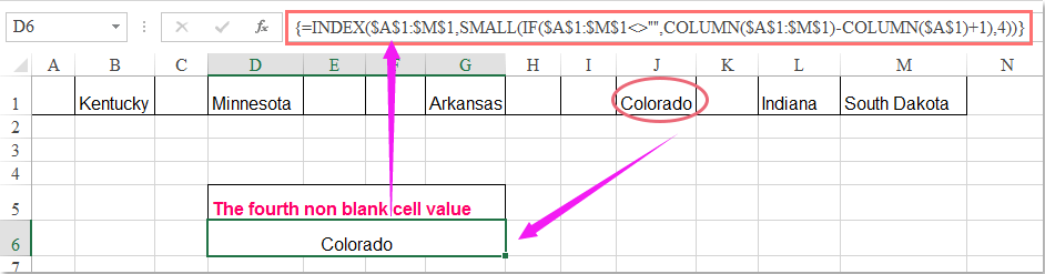
ملاحظة:في الصيغة أعلاه،A1:M1 تمثّل قيم الصف الذي تريد استخدامه، والرقم4 يشير إلى القيمة الرابعة غير الفارغة التي تريد إرجاعها. إذا كنت ترغب في الحصول على القيمة الثانية غير الفارغة، فما عليك سوى تغيير الرقم 4 إلى 2 حسب الحاجة.
أفضل أدوات الإنتاجية لمكتبتك
عزِّز مهاراتك في Excel باستخدام Kutools لـ Excel، وعايش الكفاءة كما لم تفعل من قبل.يقدّم Kutools لـ Excel أكثر من 300 ميزة متقدمة لتعزيز الإنتاجية ووقت الحفظ.انقر هنا للحصول على الميزة التي تحتاجها أكثر من غيرها...
يجلب Office Tab واجهة ذات علامات تبويب إلى Office، ويجعل عملك أسهل بكثير
- تمكّن من التحرير والقراءة باستخدام علامات التبويب في Word وExcel وPowerPoint، وPublisher وAccess وVisio وProject.
- افتح وأنشئ مستندات متعددة في علامات تبويب جديدة داخل النافذة نفسها، بدلاً من فتح نوافذ جديدة.
- يزيد إنتاجيتك بنسبة 50% ويوفّر لك مئات نقرات الفأرة كل يوم!
جميع الإضافات من Kutools في برنامج تثبيت واحد!
Kutools for Office حزمةٌ تحتوي على إضافاتٍ مخصصة لتطبيقات Excel وWord وOutlook وPowerPoint، إلى جانب Office Tab Pro، مما يجعلها الخيار المثالي للفِرق التي تعمل عبر تطبيقات Office.
- حزمة شاملة واحدة— إضافات Excel وWord وOutlook وPowerPoint بالإضافة إلى Office Tab Pro
- برنامج تثبيت واحد، ترخيص واحد— الإعداد خلال دقائق (جاهز لـ MSI)
- يعمل بشكل أفضل معًا— إنتاجية ميسَّرة عبر تطبيقات Office
- تجربة مجانية لمدة 30 يومًا بكامل الميزات— بدون تسجيل، بدون بطاقة ائتمان
- أفضل قيمة— وفِّر مقارنةً بشراء الإضافات بشكل منفصل