إنشاء مربع بحث في Excel – دليل خطوة بخطوة

يُحسّن إنشاء مربع بحث في Excel وظائف جداول البيانات لديك من خلال تسهيل تصفية البيانات والوصول إليها بسرعة. يغطي هذا الدليل عدة طرق لتنفيذ مربع بحث، لتتناسب مع إصدارات مختلفة من Excel. سواء كنت مستخدمًا مبتدئًا أو متقدمًا، ستساعدك هذه الخطوات على إعداد مربع بحث ديناميكي باستخدام ميزات مثل دالة FILTER، وتنسيق الشرط، وصيغ متنوعة.

• إنشاء مربع بحث بسهولة باستخدام دالة FILTER
  (متاحة في Excel 2019 والإصدارات الأحدث، وExcel لـ Microsoft 365)
• إنشاء مربع بحث باستخدام استخدم تنسيق الشروط
  (متاحة في جميع إصدارات Excel)
• إنشاء مربع بحث باستخدام مجموعات صيغ
  (متاحة في جميع إصدارات Excel)

إنشاء مربع بحث بسهولة باستخدام دالة FILTER

• تُحدِّث هذه الدالة الناتج تلقائيًا عند تغيير بياناتك.
• يمكن لدالة FILTER إرجاع أي عدد من النتائج—من صف واحد إلى الآلاف—بناءً على عدد الإدخالات في مجموعة البيانات التي تطابق المعايير التي حددتها.

سأوضح لك هنا كيفية استخدام دالة FILTER لإنشاء مربع بحث فعّال في Excel.

الخطوة 1: إدراج مربع نص وتكوين الخصائص

1. انتقل إلى علامة التبويب «المطور»، ثم انقر على «إدراج» > «مربع نص (عنصر تحكم ActiveX)».
   ملاحظة: إذا لم تظهر علامة التبويب «المطور» في الشريط، يمكنك تمكينها باتباع التعليمات في هذا البرنامج التعليمي:كيفية إظهار/عرض علامة تبويب المطور في شريط Excel؟
   
2. سيتحول المؤشر إلى شكل صليب؛ اسحبه بعد ذلك لرسم مربع النص في الموضع الذي تريده ضمن ورقة العمل، ثم حرّر زر الماوس بعد الانتهاء من رسم المربع.
   
3. انقر بزر الماوس الأيمن على مربع النص، ثم اختر «خصائص» من القائمة المنبثقة.
   
4. في لوحة «الخصائص»، اربط مربع النص بخلية بإدخال مرجع الخلية في حقل «LinkedCell». على سبيل المثال، يؤدي إدخال "J2" إلى تحديث أي بيانات تُدخل في مربع النص تلقائيًا في الخلية J2، والعكس بالعكس.
   
5. انقر على «وضع التصميم» في علامة التبويب «المطور» للخروج من هذا الوضع.
   

يتيح لك مربع النص الآن إدخال النص المطلوب.

الخطوة 2: تطبيق دالة FILTER

1. قبل استخدام دالة FILTER، انسخ صف العناوين الأصلي إلى منطقة جديدة. هنا، وضعتُ صف العناوين أسفل مربع البحث.
   
2. حدد الخلية الموجودة أسفل العنوان الأول (مثل I5 في هذا المثال)، وأدخل الصيغة التالية فيها ثم اضغط مفتاح «Enter» للحصول على النتيجة.

   =FILTER(Sheet2!$A$5:$G$281,Sheet2!$B$5:$B$281=J2,"No data found")

   
   كما هو موضح في لقطة الشاشة أعلاه، وبما أن مربع النص لا يحتوي الآن على أي إدخال، فإن الصيغة تعرض النتيجة «لم يتم العثور على بيانات» في الخلية I5.

النتيجة: اختبار مربع البحث

لنختبر الآن مربع البحث. في هذا المثال، بمجرد إدخالك اسم عميل في مربع البحث، سيتم تصفية النتائج ذات الصلة وعرضها فورًا.

إنشاء مربع بحث باستخدام استخدم تنسيق الشروط

يمكنك استخدام التنسيق الشرطي لتمييز البيانات التي تطابق مصطلح البحث، مما يُنشئ تأثير مربع بحث بشكل غير مباشر. هذه الطريقة لا تُصفّي البيانات، بل توجّهك بصريًا إلى الخلايا ذات الصلة. سيوضح لك هذا القسم كيفية إنشاء مربع بحث باستخدام التنسيق الشرطي في Excel.

الخطوة 1: إدراج مربع نص وتكوين الخصائص

1. انتقل إلى علامة التبويب «Developer»، وانقر فوق «Insert» > «Text Box (ActiveX Control)».
   ملاحظة: إذا لم تظهر علامة التبويب «Developer» في الشريط، يمكنك تمكينها باتباع التعليمات في هذا البرنامج التعليمي:كيفية إظهار/عرض علامة تبويب المطور في شريط Excel؟
   
2. سيتحول المؤشر إلى شكل صليب، ثم تحتاج إلى سحب المؤشر لرسم مربع النص في الموقع الذي ترغب في وضعه في ورقة العمل. بعد رسم مربع النص، حرّر زر الماوس.
   
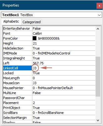
3. انقر بزر الماوس الأيمن على مربع النص، ثم اختر «الخصائص (Properties)» من القائمة السياقية.
   
4. في جزء «الخصائص» (Properties)، اربط مربع النص بخلية بإدخال مرجع الخلية في حقل «LinkedCell». على سبيل المثال، يؤدي إدخال "J3" إلى تحديث أي بيانات تُدخل في مربع النص تلقائيًا في الخلية J3، والعكس بالعكس.
   
5. انقر على «وضع التصميم» في علامة التبويب «المطور» للخروج من هذا الوضع.
   

يتيح لك مربع النص الآن إدخال النص المطلوب.

الخطوة 2: تطبيق استخدم تنسيق الشروط للبحث عن البيانات

1. حدد كامل نطاق البيانات الذي تريد البحث فيه. في هذا المثال، تم تحديد النطاق A3:G279.
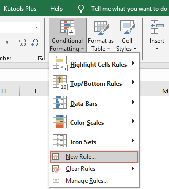
2. ضمن علامة التبويب «Home»، انقر فوق «استخدم تنسيق الشروط» > «New Rule».
   
3. في مربع حوار «New Formatting Rule»:
   1. اختر «استخدام صيغة لتحديد الخلايا التي سيتم تنسيقها» من ضمن خيارات «حدد نوع القاعدة».
   2. أدخل الصيغة التالية في مربع «تنسيق القيم حيث تكون هذه الصيغة صحيحة».

      =$B3=$J$3

      هنا، تمثّل «$B3» الخلية الأولى في العمود الذي تريد مطابقته مع معايير البحث في تحديد النطاق، و«$J$3» هي الخلية المرتبطة بمربع البحث.
   3. انقر على زر «تنسيق» لتحديد تعبئة اللون لنتائج البحث.
   4. انقر على زر «موافق». راجع لقطة الشاشة:
      

النتيجة

لنختبر الآن مربع البحث. في هذا المثال، بمجرد إدخال اسم عميل في مربع البحث، سيتم تمييز الصفوف المقابلة التي تحتوي على هذا العميل في العمود B فورًا باستخدام لون التعبئة المحدد.

إنشاء مربع بحث باستخدام مجموعات صيغ

إذا لم تكن تستخدم أحدث إصدار من Excel وتفضّل عدم الاقتصار على نطاق الصف المميز فقط، فقد تكون الطريقة الموضحة في هذا القسم مثالية لك! يمكنك الاستفادة من مجموعة من صيغ Excel لإنشاء مربع بحث فعّال يعمل بسلاسة في أي إصدار من Excel. اتبع الخطوات أدناه لتبدأ الآن.

الخطوة 1: إنشاء قائمة بالقيم الفريدة من عمود البحث

1. في هذه الحالة، قمت بتحديد ونسخ النطاق "B4:B281" إلى ورقة عمل جديدة.
2. بعد لصق النطاق في ورقة عمل جديدة، ابقِ البيانات الملصقة محددة، ثم انتقل إلى علامة التبويب «Data» وانقر على «إزالة التكرارات».
   
3. في مربع حوار «إزالة التكرارات» الذي يظهر، انقر فوق زر «موافق».
   
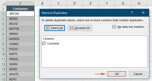
4. ثم يظهر مربع رسالة بعنوان «Microsoft Excel» يوضح عدد القيم المكررة التي تمت إزالتها. انقر فوق «موافق».
   
5. بعد إزالة القيم المكررة، حدد جميع القيم الفريدة في القائمة باستثناء العنوان، ثم عيّن اسمًا لهذا النطاق بإدخاله في مربع «Name». وقد سُمّي هذا النطاق هنا بـ «Customer».
   

الخطوة 2: إدراج مربع قائمة منسدلة وتكوين الخصائص

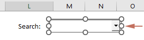
1. عُد إلى ورقة العمل التي تحتوي على مجموعة البيانات التي تريد البحث فيها. انتقل إلى علامة التبويب «Developer»، ثم انقر فوق «Insert» > «Combo Box (ActiveX Control)».
   ملاحظة: إذا لم تظهر علامة التبويب «Developer» في الشريط، يمكنك تمكينها باتباع التعليمات في هذا البرنامج التعليمي:كيفية إظهار/عرض علامة تبويب المطور في شريط Excel؟
   
2. سيتحول المؤشر إلى صليب، ثم تحتاج إلى سحب المؤشر لرسم مربع القائمة المنسدلة في الموقع الذي ترغب في وضع مربع البحث فيه بورقة العمل. بعد رسم مربع القائمة المنسدلة، حرر زر الماوس.
   
3. انقر بزر الماوس الأيمن على مربع القائمة المنسدلة، ثم اختر «Properties» من قائمة السياق.
   
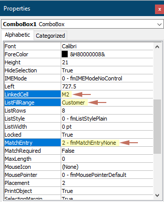
4. في جزء «الخصائص»:
   1. اربط مربع القائمة بخلية بإدخال مرجع الخلية في حقل «LinkedCell». على سبيل المثال، اكتب هنا "M2".
   2. في حقل «ListFillRange»، أدخل «اسم الخلية» الذي حددته للقائمة الفريدة في الخطوة 1.
   3. غيّر حقل «MatchEntry» إلى «2 – fmMatchEntryNone».
   4. أغلق لوحة «الخصائص».
      
5. انقر فوق «Design Mode» في علامة التبويب «Developer» للخروج من وضع التصميم.
   

يمكنك الآن اختيار أي عنصر من القائمة المنسدلة أو كتابة نص للبحث عنه بسهولة.

الخطوة 3: تطبيق الصيغ

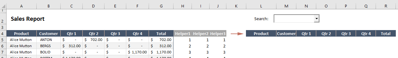
1. أنشئ ثلاثة أعمدة مساعدة بجانب نطاق البيانات الأصلي. راجع لقطة الشاشة:
   
2. في الخلية (H5) الواقعة أسفل رأس العمود المساعد الأول، أدخل الصيغة التالية ثم اضغط «Enter».

   =ROWS($B$5:B5)

   هنا، تمثّل الخلية "B5" اسم أول عميل في العمود الذي تريد البحث فيه.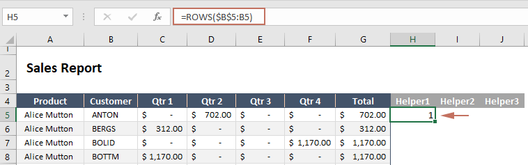
   
3. انقر مرتين على الزاوية اليمنى السفلية لخلية الصيغة، وسيتم تعبئة الخلية التالية تلقائيًا بنفس الصيغة.
   
4. في الخلية (I5) الموجودة أسفل رأس العمود المساعد الثاني، أدخل الصيغة التالية ثم اضغط «Enter». بعد ذلك، انقر نقرًا مزدوجًا على الزاوية اليمنى السفلية لخلية الصيغة لتعبئة الخلايا أدناه تلقائيًا بنفس الصيغة.

   =IF(ISNUMBER(SEARCH($M$2,B5)),H5,"")

   هنا، تمثّل الخلية "M2" الخلية المرتبطة بمربع القائمة المنسدلة.
   
5. في الخلية (J5) الموجودة أسفل رأس العمود المساعد الثالث، أدخل الصيغة التالية واضغط «Enter». ثم انقر مرتين على الزاوية اليمنى السفلية لخلية الصيغة لتعبئة الخلايا أدناه تلقائيًا بنفس الصيغة.

   =IFERROR(SMALL($I$5:$I$281,H5),"") 

   
6. انسخ صف العناوين الأصلي إلى منطقة جديدة. هنا وضعت صف العناوين أسفل مربع البحث.
   
7. حدد الخلية الواقعة أسفل العنوان الأول (مثل L5 في هذا المثال)، ثم أدخل الصيغة التالية واضغط مفتاح «Enter».

   =IFERROR(INDEX($A$5:$G$281,$J5,COLUMNS($L$4:L4)),"")

   هنا، يُمثّل "A5:G281" النطاق الكامل للبيانات التي ترغب في عرضها في خلية النتيجة.
   
8. حدد خلية الصيغة هذه، واسحب «Fill Handle» إلى اليمين ثم إلى الأسفل لتطبيق الصيغة على الأعمدة والصفوف المقابلة.
   
   ملاحظات:

   • بما أنه لا يوجد إدخال في مربع البحث، فستعرض نتائج الصيغة البيانات الخام.
   • هذه الطريقة لا تميّز بين الأحرف الكبيرة والصغيرة، مما يعني أنها ستتطابق مع النص بغض النظر عمّا إذا كتبت بالأحرف الكبيرة أو الصغيرة.

النتيجة

لنختبر الآن مربع البحث. في هذا المثال، بمجرد إدخالك أو اختيارك اسم عميل من القائمة المنسدلة، سيتم فلترة الصفوف التي تحتوي على هذا الاسم في العمود B وعرضها فورًا ضمن نطاق النتائج.

يمكن أن يؤدي إنشاء مربع بحث في Excel إلى تحسين طريقة تفاعلك مع بياناتك بشكل كبير، مما يجعل جداولك أكثر ديناميكية وسهولة في الاستخدام. سواء اخترت البساطة التي توفرها دالة FILTER، أو المساعدة البصرية من تنسيق الشروط، أو المرونة التي تقدمها تركيبات الصيغ، فإن كل طريقة توفّر أدوات قيّمة لتعزيز قدراتك في التعامل مع البيانات. جرّب هذه التقنيات لمعرفة الطريقة الأنسب لاحتياجاتك وسيناريوهات بياناتك الخاصة. ولمن يرغب في استكشاف إمكانيات Excel بشكل أعمق، يحتوي موقعنا على كنزٍ من الدروس التعليمية.اكتشف المزيد من نصائح وحيل Excel هنا.

مقالات ذات صلة