كيف يمكنك استخراج جميع السجلات بين تاريخين في Excel؟
عند العمل مع كميات كبيرة من البيانات الموسومة زمنيًّا في Excel، قد تحتاج غالبًا إلى استخراج أو تصفية جميع السجلات التي تقع بين تاريخين محددين. على سبيل المثال، قد ترغب في تحليل المعاملات خلال فترة فوترة، أو مراجعة الحضور لشهر معين، أو ببساطة فحص الإدخالات المسجّلة ضمن نطاق التاريخ مخصّص. إن البحث اليدوي ونسخ كل صف ذي صلة قد يكون أمرًا مملًّا ومعرّضًا للخطأ، خاصة مع تزايد حجم بياناتك. إن استخراج جميع السجلات بين تاريخين معيّنين بكفاءة لا يوفر وقتك وجهدك فحسب، بل يقلل أيضًا من احتمال تفويت إدخالات مهمة أو إدخال أخطاء أثناء التعامل مع البيانات.
 |  |
فيما يلي عدة طرق عملية لاستخراج جميع السجلات بين تاريخين في Excel. يتميّز كل نهج بسيناريوهات استخدامه ومزاياه الفريدة، بدءًا من الحلول القائمة على الصيغ (دون الحاجة إلى إضافات)، مرورًا بأداة Kutools for Excel لتعزيز الراحة والكفاءة، ووصولًا إلى حلول VBA والمرشّح المدمج في Excel—مما يوفّر خيارات مرنة تلائم مختلف الاحتياجات والتفضيلات.
استخراج جميع السجلات بين تاريخين باستخدام الصيغ
استخراج جميع السجلات بين تاريخين باستخدام Kutools لـ Excel![]()
استخدام VBA لاستخراج السجلات بين تاريخين
استخدام مرشّح Excel لاستخراج السجلات بين تاريخين
استخراج جميع السجلات بين تاريخين باستخدام الصيغ
لاستخراج جميع السجلات بين تاريخين في Excel باستخدام الصيغ، اتبع الخطوات التالية. يُعدّ هذا الحل مثاليًا عندما تحتاج إلى تحديث ديناميكي: إذ تتجدد النتائج تلقائيًّا كلما تغيّرت البيانات الأصلية أو شروط التواريخ. ومع ذلك، قد يبدو الإعداد الأولي معقدًا بعض الشيء إذا لم تكن معتادًا على صيغ المصفوفة، كما أن استخدامه مع مجموعات بيانات كبيرة جدًّا قد يؤدي إلى تباطؤ في أداء الحساب.
1. أنشئ ورقة عمل جديدة، مثل Sheet2، لتحديد نطاق التواريخ وعرض السجلات المستخرَجة. أدخل تاريخ البدء في الخلية A2 وتاريخ الانتهاء في الخلية B2. وللتوضيح، يمكنك إضافة عناوين في الخليتين A1 وB1 (مثل «تاريخ البدء» و«تاريخ الانتهاء»).
2. في الخلية C2 من Sheet2، أدخل الصيغة التالية لحساب عدد الصفوف في Sheet1 التي تحتوي على تواريخ تقع ضمن نطاق معيّن:
=SUMPRODUCT((Sheet1!$A$2:$A$22>=A2)*(Sheet1!$A$2:$A$22<=B2))بعد إدخال الصيغة، اضغطEnter. سيساعدك ذلك على فهم عدد الإدخالات المطابقة لشرط التصفية، مما يسهّل معرفة عدد النتائج المتوقعة.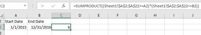
ملاحظة:في هذه الصيغة، يشيرSheet1 إلى ورقة بياناتك الأصلية؛ ويشير$A$2:$A$22 إلى عمود التواريخ في بياناتك. عدِّل هذه المراجع وفقًا لاحتياجات بياناتك. وتشيرA2 وB2 إلى خلايا تاريخ البدء وتاريخ الانتهاء.
3. لعرض السجلات المطابقة، حدد خلية فارغة لتبدأ فيها استخراج القائمة (مثلًا، الخلية A5 في Sheet2)، ثم أدخل صيغة المصفوفة التالية:
=IF(ROWS(A$5:A5)>$C$2,"",INDEX(Sheet1!A$2:A$22,SMALL(IF((Sheet1!$A$2:$A$22>=$A$2)*(Sheet1!$A$2:$A$22<=$B$2),ROW(Sheet1!A$2:A$22)-ROW(Sheet1!$A$2)+1),ROWS(A$5:A5))))بعد كتابة الصيغة، اضغطCtrl + Shift + Enter (بدلاً من مفتاح Enter وحده) لتحويلها إلى صيغة مصفوفة. بعد ذلك، استخدم مقبض التعبئة لسحب الصيغة يمينًا عبر جميع الأعمدة التي تحتوي على بيانات، ثم لأسفل حتى تظهر كل الصفوف المطابقة. استمر بالسحب حتى تبدأ الخلايا الفارغة بالظهور—وهو مؤشر على أن جميع البيانات المطابقة قد تم استخراجها بالكامل.
نصائح:
- إذا ظهرت لك أصفار، فهذا يعني أنه لا توجد سجلات مطابقة إضافية لإرجاعها؛ لذا ما عليك سوى التوقف عن السحب أكثر من ذلك.
- يمكنك تعديل الجزءINDEX(...) من الصيغة لاستخراج أعمدة أخرى. غيّر العمود المرجعي في الجزءSheet1!A$2:A$22 إذا كنت ترغب في إرجاع حقول أخرى.
- يمكن توسيع هذه الصيغة للعمل مع معايير متعددة أو لاستخراج الصف بأكمله (بمجرد تكرارها في كل عمود).
4. قد تظهر بعض نتائج التواريخ كأرقام مكوَّنة من 5 أرقام (وهي أرقام التواريخ التسلسلية في Excel). لتحويلها إلى تنسيق تاريخ مقروء، حدد الخلايا المطلوبة، ثم انتقل إلى علامة التبويبالصفحة الرئيسية، وافتح قائمة التنسيق المنسدلة، واخترتاريخ قصير. بهذه الطريقة، تصبح البيانات المستخرَجة أكثر وضوحًا وسهولة في الاستخدام.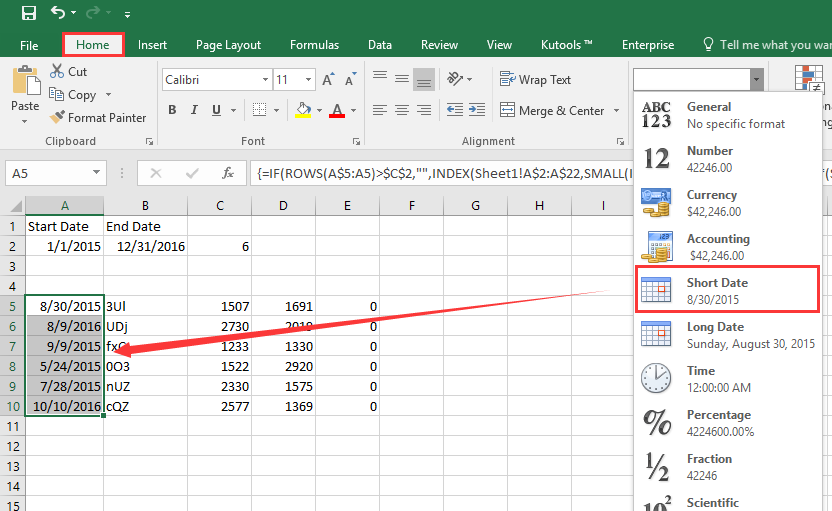
احتياطات:
- تأكد من أن جميع إدخالات التواريخ في بياناتك الأصلية موجودة فعليًّا بتنسيق التاريخ، وليس محفوظة كنص؛ وإلا فقد لا تعمل الصيغة كما هو متوقع.
- عدِّل نطاقات المصفوفة عند تغيُّر حجم بياناتك.
- إذا ظهرت أخطاء مثل #NUM! أو #N/A، فتحقق من وجود تواريخ فارغة أو عدم اتساق في البيانات الأصلية.
استخراج جميع السجلات بين تاريخين باستخدام Kutools لـ Excel
إذا كنت تفضل حلاً أكثر سلاسة وتفاعلاً، فإن ميزةتحديد خلايا محددةفي Kutools لـ Excel تساعدك على استخراج الصف بأكمله الذي يطابق نطاق التاريخ الخاص بك بنقرات قليلة فقط، مما يقلل الحاجة إلى الصيغ أو الإعداد اليدوي. وهي مثالية بشكل خاص للمستخدمين الذين يتعاملون غالبًا مع مهام تصفية معقدة أو يُجرون عمليات دفعية على مجموعات بيانات كبيرة، إذ تقلل من احتمال حدوث أخطاء في الصيغ وتساعد على تسريع سير العمل.
بعد تثبيتKutools لـ Excel، يُرجى اتباع الخطوات التالية:(تنزيل مجاني لـ Kutools لـ Excel الآن!)
1. أولًا، حدد نطاق مجموعة البيانات التي ترغب في تحليلها واستخراج البيانات منها. بعد ذلك، انقر فوقKutools > تحديد > تحديد خلايا محددةمن شريط Excel. وسيؤدي ذلك إلى فتح نافذة حوار للاختيار المتقدم.
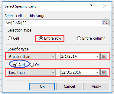
2. في نافذة الحوارتحديد خلايا محددة:
- فعّل خيار «الصف بأكمله» لتحديد الصفوف المطابقة بالكامل.
- اضبط شرط التصفية: اختر أكبر من وأصغر من في القائمة المنسدلة الخاصة بعمود التواريخ.
- أدخل يدويًّا تاريخ البدء وتاريخ الانتهاء في مربع النص، مع التأكد من أن التنسيق يتوافق مع بياناتك.
- تأكد من اختيار منطق «و» (And) لتطبيق الشرطين معًا في آنٍ واحد.
3. انقر فوقموافق. سيقوم Kutools فورًا بتحديد جميع الصفوف التي يقع عمود التاريخ فيها ضمن النطاق المحدود الذي حددته. بعد ذلك، اضغطCtrl + C لنسخ الصفوف المحددة، ثم انتقل إلى ورقة فارغة أو موقع جديد، واضغطCtrl + V للصق النتائج المستخرَجة.
نصائح وتحذيرات:
- نهج Kutools لا يتطلب تعديل بياناتك الأصلية أو كتابة أي صيغ.
- إذا واجهت أي مشكلات في تنسيق التاريخ، فتأكد من مراجعة نتائج التحديد قبل النسخ.
- استخدم هذه الميزة للمهام المتكررة أو الدُفعات (batch)—فهي تتيح لك تكرار الخطوات بسرعة عبر نطاق التواريخ المختلفة.
- إذا لم تظهر الميزة في إصدار Kutools الخاص بك كما هو موصوف، فقم بالتحديث إلى أحدث إصدار لضمان أفضل توافق.
تحليل السيناريوهات:هذه الطريقة مثالية للمستخدمين الذين يديرون قوائم ذات أعمدة عديدة، أو لأولئك الذين يحتاجون إلى استخراج سجلات كاملة بشكل متكرر بناءً على تواريخ حدودية متغيرة.
رمز VBA - استخدام ماكرو لتصفية واستخراج جميع الصفوف تلقائيًا بين تاريخين تاريخ محدد
إذا كان سير عملك يتضمّن غالبًا استخراج بيانات بين تاريخين وتسعى إلى أتمتة العملية بالكامل، فإن استخدام ماكرو VBA يُعد خيارًا ذكيًّا. فباستخدام VBA، يمكنك مطالبة المستخدمين باختيار عمود التاريخ، وإدخال تاريخ البدء وتاريخ الانتهاء، ثم تصفية الصفوف المطابقة ونسخها تلقائيًّا إلى ورقة جديدة. هذه الطريقة توفر الجهد اليدوي وتقلّل الأخطاء، لكنها تتطلب تمكين الماكروات وبعض الإلمام بمحرّر Visual Basic.
إليك كيفية إعداد هذا الماكرو:
1. انقر فوقالمطور > Visual Basic لفتح محرر VBA. في نافذةMicrosoft Visual Basic for Applications الجديدة، انقر فوقإدراج > وحدة، ثم انسخ والصق الكود التالي في الوحدة:
Sub ExtractRowsBetweenDates_Final()
'Updated by Extendoffice
    Dim wsSrc As Worksheet
    Dim wsDest As Worksheet
    Dim rngTable As Range
    Dim colDate As Range
    Dim StartDate As Date
    Dim EndDate As Date
    Dim i As Long
    Dim destRow As Long
    Dim dateColIndex As Long
    Dim cellDate As Variant

    Set wsSrc = ActiveSheet
    Set rngTable = Application.InputBox("Select the data table (including headers):", "KutoolsforExcel", Type:=8)
    If rngTable Is Nothing Then Exit Sub

    Set colDate = Application.InputBox("Select the date column (including header):", "KutoolsforExcel", Type:=8)
    If colDate Is Nothing Then Exit Sub

    On Error GoTo DateError
    StartDate = CDate(Application.InputBox("Enter the start date (yyyy-mm-dd):", "KutoolsforExcel", "", Type:=2))
    EndDate = CDate(Application.InputBox("Enter the end date (yyyy-mm-dd):", "KutoolsforExcel", "", Type:=2))
    On Error GoTo 0

    On Error Resume Next
    Set wsDest = Worksheets("FilteredRecords")
    On Error GoTo 0
    If wsDest Is Nothing Then
        Set wsDest = Worksheets.Add
        wsDest.Name = "FilteredRecords"

        rngTable.Rows(1).Copy
        wsDest.Cells(1, 1).PasteSpecial Paste:=xlPasteValuesAndNumberFormats
        wsDest.Cells(1, 1).PasteSpecial Paste:=xlPasteFormats
    End If

    destRow = wsDest.Cells(wsDest.Rows.Count, 1).End(xlUp).Row + 1
    dateColIndex = colDate.Column - rngTable.Columns(1).Column + 1

    For i = 2 To rngTable.Rows.Count
        cellDate = rngTable.Cells(i, dateColIndex).Value
        If IsDate(cellDate) Then
            If cellDate >= StartDate And cellDate <= EndDate Then
                rngTable.Rows(i).Copy
                wsDest.Cells(destRow, 1).PasteSpecial Paste:=xlPasteValuesAndNumberFormats
                wsDest.Cells(destRow, 1).PasteSpecial Paste:=xlPasteFormats
                destRow = destRow + 1
            End If
        End If
    Next i

    Application.CutCopyMode = False
    wsDest.Columns.AutoFit
    MsgBox "Filtered results have been added to '" & wsDest.Name & "'.", vbInformation
    Exit Sub

DateError:
    MsgBox "Invalid date format. Please enter dates as yyyy-mm-dd.", vbExclamation
End Sub
2. لتشغيل الماكرو، انقر فوق زر![]() (تشغيل) أو اضغطF5.
(تشغيل) أو اضغطF5.
ثم اتبع التعليمات لإكمال الخطوات:
- حدد جدول البيانات (بما في ذلك العناوين)عند ظهور مربع الإدخال الأول، حدد الجدول بأكمله بما في ذلك صف العناوين، ثم انقرموافق.
- حدد عمود التواريخ (بما في ذلك العنوان)عند ظهور مربع الإدخال الثاني، حدد عمود التواريخ فقط بما في ذلك العنوان، ثم انقرموافق.
- أدخل تاريخ البدء وتاريخ الانتهاءسيُطلب منك إدخال تاريخ البدء (التنسيق: yyyy-mm-dd، مثال: 2025-06-01)ثم أدخل تاريخ الانتهاء (مثال: 2025-06-30)وانقرموافقبعد كل إدخال.
سيتم إنشاء ورقة عمل باسم FilteredRecords تلقائيًا (في حال لم تكن موجودة مسبقًا)، ويتم نسخ الصفوف المطابقة—التي يقع تاريخها بين تاريخ البدء وتاريخ الانتهاء—إلى تلك الورقة. وفي كل مرة تُشغّل فيها الماكرو، ستُلحَق أي صفوف مطابقة جديدة أسفل النتائج الموجودة.
استكشاف الأخطاء وإصلاحها:
- إذا لم يحدث شيء بعد التشغيل، فتأكد من أن النطاق المحدد صحيح—فأي نطاق غير صالح أو إلغاء مربعات الحوار سيؤدي إلى إنهاء الماكرو.
- تأكد من أن إدخالات عمود التواريخ هي تواريخ Excel حقيقية؛ وإذا كانت محفوظة كنص، فحوّلها أولًا لضمان تصفية دقيقة.
تحليل السيناريوهات:يُعدّ هذا الحل المبني على VBA مثاليًا خصوصًا للمهام المتكررة أو سير العمل المتقدم، وكذلك عند مشاركة حل شبه آلي مع مستخدمين غير تقنيين—فكل ما عليك هو تعيين زر لتبسيط التشغيل!
طرق Excel المدمجة الأخرى - استخدام ميزة التصفية المدمجة في Excel
للمستخدمين الذين يفضلون نهجًا تفاعليًا بسيطًا دون الحاجة إلى كتابة صيغ أو أكواد، توفّر ميزة التصفية المدمجة في Excel وسيلة سريعة لعرض واستخراج الصفوف الواقعة بين تاريخين. وهي مثالية للمهام العرضية أو الفحص البصري أو عند الرغبة في العمل مباشرةً من خلال واجهة الورقة. ومع ذلك، لا تدعم هذه الميزة تحديثات تلقائية عند تغيّر معايير التواريخ أو البيانات—بل يتطلب الأمر تكرار خطوات التصفية يدويًّا في كل مرة.
إليك كيفية استخدامها:
- حدد نطاق بياناتك، مع التأكد من تضمين عناوين الأعمدة.
- انتقل إلى علامة التبويببياناتفي الشريط، ثم انقرتصفية. ستظهر سهام صغيرة للقائمة المنسدلة بجانب كل عنوان.
- انقر على السهم بجانب عمود التواريخ، ثم اخترمرشحات التاريخ > بين....
- في مربع الحوار، أدخل تاريخ البدء وتاريخ الانتهاء المطلوبين، وتأكد من أن تنسيقهُما يطابق تنسيق التاريخ المستخدم في بياناتك.
- انقرموافق، وسيتم عرض الصفوف التي تحتوي على تواريخ ضمن النطاق المحدد من قِبَلك فقط.
- حدد جميع الصفوف المرئية، ثم اضغطCtrl + C لنسخها. بعد ذلك، انتقل إلى منطقة فارغة أو ورقة أخرى، واضغطCtrl + V لصق نتائج التصفية.
نصائح واحتياطات:
- هذه الطريقة مثالية للمراجعة البصرية السريعة أو الاستخراج العرضي.
- إذا كان عمود التواريخ يحتوي على تنسيقات غير متناسقة، فقم بتصحيحها مسبقًا لضمان عمل المرشِّح بدقة.
- لا تنسَ إزالة التصفية عند الانتهاء لإعادة عرض مجموعة البيانات الكاملة.
- الصفوف المُرشَّحة تكون مخفية، وليس محذوفة—فبياناتك الأصلية تظل سليمة.
تحليل السيناريوهات:تُعد ميزة التصفية المدمجة في Excel الخيار الأنسب للجداول ذات الحجم المتوسط، خاصةً عندما تحتاج إلى معاينة فورية أو نسخ مجموعات فرعية دون الحاجة إلى حفظ صيغ أو ماكروات.
استكشاف الأخطاء وإصلاحها واقتراحات الخلاصة:
- تأكد دائمًا من تنسيق خلايا التواريخ بشكل متناسق عبر ورقة العمل بأكملها لضمان عمل جميع الحلول كما يجب.
- عند استخدام الصيغ أو VBA، تأكد من تعديل مراجع الأعمدة والنطاقات لتتماشى مع البنية الفعلية لورقتك، وتجنب بذلك أخطاء الفهرسة أو المرجع.
- من حيث الأداء على مجموعات البيانات الكبيرة جدًّا، عادةً ما يوفّر Kutools أو التصفية المدمجة نتائج أسرع، ويكون من غير المرجّح أن تتجاوز حدود الذاكرة أو حساب الصيغ مقارنةً باستخدام صيغ مصفوفة موسّعة.
- إذا واجهت خلايا فارغة غير متوقعة أو سجلات مفقودة في الناتج، فتأكد من ضبط شروط التواريخ ونطاق الإدخال وتنسيقات البيانات بالشكل الذي تريده.
عرض توضيحي: استخراج جميع السجلات بين تاريخين باستخدام Kutools لـ Excel
أفضل أدوات الإنتاجية لمكتبتك
عزِّز مهاراتك في Excel باستخدام Kutools لـ Excel، وعايش الكفاءة كما لم تفعل من قبل.يقدّم Kutools لـ Excel أكثر من 300 ميزة متقدمة لتعزيز الإنتاجية ووقت الحفظ.انقر هنا للحصول على الميزة التي تحتاجها أكثر من غيرها...
يجلب Office Tab واجهة ذات علامات تبويب إلى Office، ويجعل عملك أسهل بكثير
- تمكّن من التحرير والقراءة باستخدام علامات التبويب في Word وExcel وPowerPoint، وPublisher وAccess وVisio وProject.
- افتح وأنشئ مستندات متعددة في علامات تبويب جديدة داخل النافذة نفسها، بدلاً من فتح نوافذ جديدة.
- يزيد إنتاجيتك بنسبة 50% ويوفّر لك مئات نقرات الفأرة كل يوم!
جميع الإضافات من Kutools في برنامج تثبيت واحد!
Kutools for Office حزمةٌ تحتوي على إضافاتٍ مخصصة لتطبيقات Excel وWord وOutlook وPowerPoint، إلى جانب Office Tab Pro، مما يجعلها الخيار المثالي للفِرق التي تعمل عبر تطبيقات Office.
- حزمة شاملة واحدة— إضافات Excel وWord وOutlook وPowerPoint بالإضافة إلى Office Tab Pro
- برنامج تثبيت واحد، ترخيص واحد— الإعداد خلال دقائق (جاهز لـ MSI)
- يعمل بشكل أفضل معًا— إنتاجية ميسَّرة عبر تطبيقات Office
- تجربة مجانية لمدة 30 يومًا بكامل الميزات— بدون تسجيل، بدون بطاقة ائتمان
- أفضل قيمة— وفِّر مقارنةً بشراء الإضافات بشكل منفصل