كيف تُنشئ قائمة منسدلة معتمدة في Google Sheets؟
قد يكون إدراج قائمة منسدلة عادية في Google Sheets أمرًا سهلاً بالنسبة لك، لكنك أحيانًا قد تحتاج إلى إنشاء قائمة منسدلة ديناميكية، بحيث تعتمد القائمة الثانية على الخيار المحدد في القائمة الأولى. كيف يمكنك تنفيذ هذه المهمة في Google Sheets؟
إنشاء قائمة منسدلة معتمدة في Google Sheets
إنشاء قائمة منسدلة معتمدة في Google Sheets
اتبع هذه الخطوات لإنشاء قائمة ديناميكية في Google Sheets:
1. أولًا، أدرج القائمة المنسدلة الأساسية: اختر الخلية التي تريد وضع القائمة المنسدلة الأولى فيها، ثم انقرالبيانات > التحقق من صحة البيانات. انظر لقطة الشاشة:

2. في مربع الحوار المنبثقالتحقق من صحة البيانات، اخترقائمة من نطاقمن القائمة المنسدلة بجانب قسمالمعايير، ثم انقر على الزر لتحديد قيم الخلايا التي تريد إنشاء القائمة المنسدلة الأولى بناءً عليها. انظر لقطة الشاشة: 

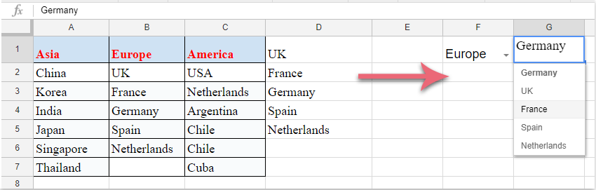
3. بعد ذلك، انقر على زرحفظ. عندئذٍ، تكون القائمة المنسدلة الأولى قد أُنشئت. اختر عنصرًا واحدًا من القائمة المنسدلة التي تم إنشاؤها، ثم أدخل هذه الصيغة: =arrayformula(if(F1=A1,A2:A7,if(F1=B1,B2:B6,if(F1=C1,C2:C7,«»)))) في خلية فارغة مجاورة لأعمدة البيانات، ثم اضغط على مفتاحإدخال. ستُعرض جميع القيم المطابقة استنادًا إلى عنصر القائمة المنسدلة الأولى دفعة واحدة. انظر لقطة الشاشة:
ملاحظة: في الصيغة أعلاه،F1 هي خلية القائمة المنسدلة الأولى، وA1 وB1 وC1 هي عناصر القائمة المنسدلة الأولى، بينماA2:A7 وB2:B6 وC2:C7 هي قيم الخلايا التي تستند إليها القائمة المنسدلة الثانية. يمكنك تغييرها حسب بياناتك الخاصة.

4. بعد ذلك، لإنشاء القائمة المنسدلة المعتمدة الثانية، انقر على الخلية التي تريد وضع القائمة المنسدلة الثانية فيها، ثم انتقل إلىالبيانات > التحقق من صحة البياناتلفتح مربع حوارالتحقق من صحة البيانات. من القائمة المنسدلة بجانب قسمالمعايير، اخترقائمة من نطاق، ثم انقر على الزر لتحديد خلايا الصيغة التي تمثّل نتائج المطابقة الخاصة بالعنصر المحدد في القائمة المنسدلة الأولى. انظر لقطة الشاشة:

5. وأخيرًا، انقر على زر الحفظ. وبذلك تكون القائمة المنسدلة المعتمدة الثانية قد أُنشئت بنجاح، كما هو موضح في لقطة الشاشة التالية:
أفضل أدوات الإنتاجية لمكتبتك
عزِّز مهاراتك في Excel باستخدام Kutools لـ Excel، وعايش الكفاءة كما لم تفعل من قبل.يقدّم Kutools لـ Excel أكثر من 300 ميزة متقدمة لتعزيز الإنتاجية ووقت الحفظ.انقر هنا للحصول على الميزة التي تحتاجها أكثر من غيرها...
يجلب Office Tab واجهة ذات علامات تبويب إلى Office، ويجعل عملك أسهل بكثير
- تمكّن من التحرير والقراءة باستخدام علامات التبويب في Word وExcel وPowerPoint، وPublisher وAccess وVisio وProject.
- افتح وأنشئ مستندات متعددة في علامات تبويب جديدة داخل النافذة نفسها، بدلاً من فتح نوافذ جديدة.
- يزيد إنتاجيتك بنسبة 50% ويوفّر لك مئات نقرات الفأرة كل يوم!
جميع الإضافات من Kutools في برنامج تثبيت واحد!
Kutools for Office حزمةٌ تحتوي على إضافاتٍ مخصصة لتطبيقات Excel وWord وOutlook وPowerPoint، إلى جانب Office Tab Pro، مما يجعلها الخيار المثالي للفِرق التي تعمل عبر تطبيقات Office.
- حزمة شاملة واحدة— إضافات Excel وWord وOutlook وPowerPoint بالإضافة إلى Office Tab Pro
- برنامج تثبيت واحد، ترخيص واحد— الإعداد خلال دقائق (جاهز لـ MSI)
- يعمل بشكل أفضل معًا— إنتاجية ميسَّرة عبر تطبيقات Office
- تجربة مجانية لمدة 30 يومًا بكامل الميزات— بدون تسجيل، بدون بطاقة ائتمان
- أفضل قيمة— وفِّر مقارنةً بشراء الإضافات بشكل منفصل