كيف يمكنني استخدام التنسيق الشرطي استنادًا إلى ورقة أخرى في جدول بيانات Google؟
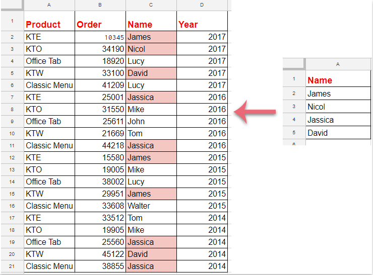
تُعد ميزة التنسيق الشرطي في Google Sheets أداة قوية تتيح لك تمييز الخلايا تلقائيًا وفقًا لمعايير محددة، مما يسهل تحليل البيانات وتصورها بسلاسة. في بعض الأحيان، بدلًا من الاعتماد على القيم الموجودة في نفس الورقة، قد تحتاج إلى ربط قواعد التنسيق الشرطي بقائمة مرجعية أو معايير مخزَّنة في ورقة مختلفة. على سبيل المثال، قد ترغب في تمييز خلايا في ورقة ما إذا كانت قيمتها موجودة أيضًا في قائمة محفوظة في ورقة أخرى، كما يظهر في لقطة الشاشة أدناه. يُعد هذا النوع من السيناريوهات شائعًا عند التعامل مع بيانات متقاطعة، مثل مقارنة مبيعات حالية بقائمة منتجات رئيسية، أو التحقق من وجود إدخالات مكررة مقابل نطاق مصدر خارجي. ومع ذلك، قد يبدو إعداد تنسيق شرطي كهذا في Google Sheets—خاصة عند الرجوع إلى بيانات عبر أوراق متعددة—محيرًا بعض الشيء إذا لم تجرِّبه من قبل. ولحسن الحظ، سيوضح لك الدليل أدناه، خطوة بخطوة، طريقة مباشرة وفعّالة لتحقيق ذلك.
طريقة تمييز الخلايا استنادًا إلى قائمة من ورقة أخرى في Google Sheets
تعليمات تمييز الخلايا استنادًا إلى قائمة من ورقة أخرى في Google Sheets
تسمح لك هذه الطريقة بإنشاء قاعدة تنسيق شرطي لتمييز الخلايا في ورقة العمل الحالية إذا ظهرت في قائمة معيّنة من ورقة أخرى. ويُعد هذا النوع من التنسيق الشرطي بين الأوراق مفيدًا بشكل خاص لمراقبة البيانات الديناميكية والحفاظ على الاتساق بين مجموعات البيانات المرتبطة.
لمتابعة هذه العملية، اتبع الخطوات التفصيلية التالية:
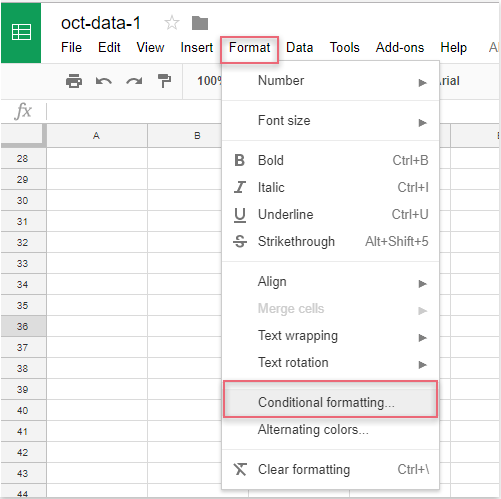
1. افتح ورقة العمل المستهدفة، ثم انقر على قائمةتنسيقفي الأعلى، واختراستخدم تنسيق الشروط. ستظهر لوحةقواعد تنسيق شرطيعلى الجانب الأيمن من شاشتك.
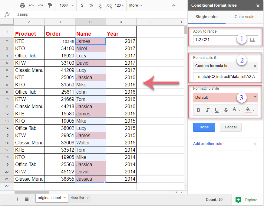
2. في لوحةقواعد التنسيق الشرطي، قم بالإجراءات التالية:
(1.) انقر على الزر المجاور لحقل «تطبيق على النطاق»، ثم حدد نطاق الخلايا التي ترغب في تنسيقها. على سبيل المثال، إذا كنت تريد تنسيق جميع القيم في العمود C بدءًا من الصف 2 فما دون، فحدّدC2:C. ويضمن تحديد النطاق المناسب تقييم الخلايا المقصودة فقط للتنسيق.
(2.) في قائمةالتنسيق إذاالمنسدلة، اخترصيغة مخصصة هي. أدخل الصيغة التالية في المربع المخصص:=match(C2,indirect(«data list!A2:A»),0). تتحقق هذه الصيغة مما إذا كانت كل خلية في العمود C تطابق أي قيمة في النطاق A2:A من ورقة «قائمة البيانات».
(3.) ضمننمط التنسيق، اختر التنسيق الذي تريده—مثل تعبئة الخلية بلون معيّن أو تغيير نمط الخط—ويمكنك معاينة النمط فورًا في ورقتك قبل تطبيقه.
ملاحظة: في الصيغة أعلاه، يشيرC2 إلى الخلية الأولى في نطاق تحديدها (عدّلها إذا كانت بياناتك تبدأ من صف أو عمود مختلف)، ويشيرقائمة البيانات!A2:Aإلى اسم الورقة («قائمة البيانات») والنطاق المقابل (A2:A) الذي يتم فيه تخزين قائمتك من الورقة الأخرى. تأكد من أن مرجع الخلية في الصيغة يطابق الخلية العلوية اليسرى في نطاق تحديدها، وإلا فقد لا يُطبَّق التنسيق بشكل صحيح. وإذا كان نطاق قائمة البيانات لديك مختلفًا، فلا تنسَ تحديثه في الصيغة (مثلًا: «قائمة البيانات!B2:B»).
3. بمجرد إعداد القاعدة، سيتم تمييز الخلايا المطابقة في النطاق الذي اخترته فورًا بناءً على القائمة من الورقة الأخرى. راجع المعاينة، ثم انقر علىتمفي أسفل لوحةقواعد التنسيق الشرطيلتطبيق التنسيق وحفظه.
نصائح واستكشاف الأخطاء وإصلاحها:
- راجع صياغتك بعناية بحثًا عن الأخطاء الإملائية، خاصةً في أسماء الأوراق ومراجع النطاقات؛ إذ تُعد المراجع غير الصحيحة سببًا شائعًا لفشل تطبيق القواعد.
- إذا احتوت قائمة بياناتك على خلايا فارغة، فإن دالة
MATCHسترجع خطأً#N/Aللقيم غير المطابقة، لكن هذا سلوكٌ متوقع ولا يؤثر على تمييز العناصر المطابقة. - عند نسخ التنسيق إلى ورقة جديدة أو تعديل النطاقات، تأكد من تحديث مراجع الخلايا في صيغتك المخصصة وفقًا لذلك.
- يتم تحديث التنسيق تلقائيًا إذا قمت لاحقًا بإضافة عناصر إلى قائمة المرجع الخاصة بك أو حذفها منها.
- الورقة والنطاق المشار إليهما في صيغتك موجودان ومكتوبان بشكلٍ صحيح.
- الخلية الأولى في صيغتك تطابق الخلية الأولى ضمن نطاق التحديد.
- تتوفر جميع الأذونات المطلوبة للوصول بين الأوراق داخل جدول البيانات الخاص بك—فهذه الطريقة تعمل ضمن ملف واحد متعدد الأوراق من Google Sheets، وليس عبر ملفات منفصلة.
كحل بديل، إذا كان هيكل بياناتك أو متطلباتك أكثر تعقيدًا—مثلًا، إذا احتجتَ إلى مقارنة أعمدة متعددة، أو السماح بمطابقات جزئية، أو تنفيذ عمليات بحث متقدمة—فيمكنك استخدام أعمدة مساعدة تحتوي على صيغCOUNTIF أوVLOOKUP، أو حتى اللجوء إلى برنامج نصي مخصص عبر Google Apps Script (كود JavaScript مخصص) لتحقيق حلول مرنة باستخدام التنسيق الشرطي.
باختصار، يُعد إعداد «استخدم تنسيقًا شرطيًّا استنادًا إلى ورقة أخرى» في Google Sheets أداةً فعّالة للغاية للتحقق من القوائم، وتتبُّع القيم المتكررة، وإجراء مختلف عمليات التحقق من البيانات بين الأوراق. تأكد دائمًا من صحة صيغتك، ونطاقات المرجع، وقواعد التنسيق للحصول على نتائج دقيقة وسلسة.

افتح سحر إكسل مع KUTOOLS AI
- التنفيذ الذكي: نفِّذ عمليات الخلايا، وحلِّل البيانات، وأنشئ المخططات البيانية — كل ذلك بأوامر بسيطة!
- الصيغ المخصصة: أنشئ صيغًا مخصصة لتبسيط سير عملك.
- برمجة VBA: اكتب وأَنفِذ أكواد VBA بسلاسة تامة.
- تفسير الصيغ: افهم الصيغ المعقدة بسهولة!
- ترجمة النصوص: اكسر الحواجز اللغوية في جداولك الإلكترونية!
أفضل أدوات الإنتاجية لمكتبتك
عزِّز مهاراتك في Excel باستخدام Kutools لـ Excel، وعايش الكفاءة كما لم تفعل من قبل.يقدّم Kutools لـ Excel أكثر من 300 ميزة متقدمة لتعزيز الإنتاجية ووقت الحفظ.انقر هنا للحصول على الميزة التي تحتاجها أكثر من غيرها...
يجلب Office Tab واجهة ذات علامات تبويب إلى Office، ويجعل عملك أسهل بكثير
- تمكّن من التحرير والقراءة باستخدام علامات التبويب في Word وExcel وPowerPoint، وPublisher وAccess وVisio وProject.
- افتح وأنشئ مستندات متعددة في علامات تبويب جديدة داخل النافذة نفسها، بدلاً من فتح نوافذ جديدة.
- يزيد إنتاجيتك بنسبة 50% ويوفّر لك مئات نقرات الفأرة كل يوم!
جميع الإضافات من Kutools في برنامج تثبيت واحد!
Kutools for Office حزمةٌ تحتوي على إضافاتٍ مخصصة لتطبيقات Excel وWord وOutlook وPowerPoint، إلى جانب Office Tab Pro، مما يجعلها الخيار المثالي للفِرق التي تعمل عبر تطبيقات Office.
- حزمة شاملة واحدة— إضافات Excel وWord وOutlook وPowerPoint بالإضافة إلى Office Tab Pro
- برنامج تثبيت واحد، ترخيص واحد— الإعداد خلال دقائق (جاهز لـ MSI)
- يعمل بشكل أفضل معًا— إنتاجية ميسَّرة عبر تطبيقات Office
- تجربة مجانية لمدة 30 يومًا بكامل الميزات— بدون تسجيل، بدون بطاقة ائتمان
- أفضل قيمة— وفِّر مقارنةً بشراء الإضافات بشكل منفصل