كيف يمكن إرجاع قيمة ما إذا وُجدت قيمة معيّنة ضمن نطاق محدّد في Excel؟
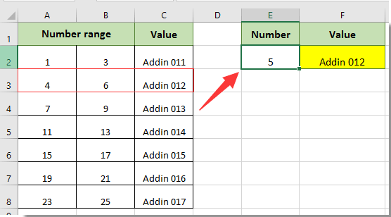
عند العمل مع البيانات في Excel، غالبًا ما يكون من الضروري تحديد ما إذا كانت قيمة معيّنة موجودة ضمن نطاق محدّد، وإذا كانت كذلك، استرجاع قيمة من خلية مجاورة تتوافق مع تلك القيمة. على سبيل المثال، كما هو موضح في لقطة الشاشة على اليسار، إذا كنت تبحث عن الرقم 5 ضمن قائمة أو نطاق، فقد ترغب في إرجاع القيمة المجاورة المقابلة تلقائيًا – وهو أمر مفيد في مهام مثل البحث عن معرّفات المنتجات، أو استرجاع معلومات المستخدمين، أو مطابقة الرموز بالقيم دون بحث يدوي.
إرجاع قيمة إذا كانت قيمة معيّنة موجودة في نطاق معيّن
إرجاع قيمة إذا كانت قيمة معيّنة موجودة في نطاق معيّن باستخدام دالة VLOOKUP
للاسترجاع السريع لقيمة مرتبطة بإدخال معيّن من جدول بيانات أو نطاق في Excel، توفّر دالةVLOOKUP حلاً مباشرًا.
هذه الطريقة فعّالة بشكل خاص إذا كان عمود البحث (حيث تبحث عن القيمة) هو العمود الأيسر في نطاق البيانات، وأردت إرجاع بيانات من عمود يقع على يمينه. وهي المستخدمة بشكل متكرر للبحث عن الرموز أو الأسماء أو المعرّفات أو أرقام المرجع واسترجاع التفاصيل ذات الصلة بسهولة.
1. حدد الخلية الفارغة التي ترغب في عرض الناتج فيها، ثم أدخل الصيغة التالية في شريط الصيغة:
=VLOOKUP(E2,A2:C8,3,TRUE)اضغطEnter لتنفيذ الصيغة. انظر لقطة الشاشة:
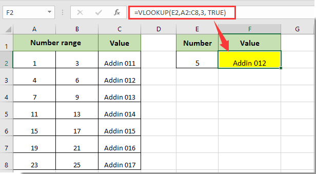
في هذا المثال، إذا وُجد الرقم 5 (في الخلية E2) ضمن النطاق المحدد في العمود A (مثلًا بين 4 و6)، سيبحث Excel عن هذه القيمة ويُدخل تلقائيًا القيمة المقابلة من العمود الثالث (العمود C) في النطاق A2:C8 إلى الخلية المحددة. وفي الرسم التوضيحي، يُعاد "Addin 012" لأن الرقم 5 يقع ضمن النطاق 4–6.
ملاحظة:في الصيغة، يشيرE2 إلى قيمة البحث، ويشكّلA2:C8 نطاق البيانات الذي يشمل كلًّا من عمود قيمة البحث والأعمدة التي تحتوي على القيم المراد إرجاعها، بينما يُحدّد الرقم3 أن القيمة المُعادة يجب أن تأتي من العمود الثالث ضمن هذا النطاق. قم بتعديل هذه المراجع لتناسب ورقة العمل الخاصة بك.
نصائح وأخطاء شائعة:
- تأكد من أن نطاق البحث (A2:C8) يشمل عمود البحث وعمود القيمة المراد إرجاعها.
- عند استخدام VLOOKUP مع المعاملTRUE، يجب أن يكون عمود البحثمرتّبًا بترتيب تصاعدي، وإلا فقد تحصل على نتائج غير متوقعة.
- للمطابقة الدقيقة، استخدمFALSE كمعامل رابع، ولكن للبحث ضمن نطاق (كما في هذا المثال)، اتركه كـTRUE.
- إذا كانت بياناتك تتغيّر باستمرار، فتأكد من مراجعة مراجعك مرة أخرى لتجنب أخطاء عدم المحاذاة.
إرجاع قيمة إذا كانت قيمة معيّنة موجودة في نطاق معيّن باستخدام دوال INDEX وMATCH
إندمج دالتَي INDEX وMATCHطريقة مرنة لإرجاع قيمة عندما تكون قيمة معيّنة موجودة في نطاق معيّن. وعلى عكس VLOOKUP، يمكن لـ INDEX وMATCH البحث عن قيمة في أي عمود وإرجاع نتيجة من أي عمود آخر، بغض النظر عن ترتيب الأعمدة. وهذا مفيد بشكل خاص إذا لم يكن عمود البحث هو العمود الأيسر أو إذا احتجتَ إلى مزيد من المرونة في هيكل بياناتك.
1. حدد خلية فارغة تريد أن يظهر فيها الناتج (مثلًا، F2)، ثم أدخل الصيغة التالية في شريط الصيغة:
=INDEX(C2:C8, MATCH(E2, A2:A8,1))اضغطEnter لتأكيد الصيغة.
- MATCH(E2, A2:A8, 1) يبحث عن موضع أكبر قيمة أقل من أو تساوي E2 في العمود A. (يتطلب ذلك أن يكون العمود A مرتبًا بترتيب تصاعدي.)
- INDEX(C2:C8, ...) يُرجع القيمة من العمود C بناءً على رقم الصف الذي يحدده MATCH.
تبحث هذه الصيغة عن القيمة فيE2 ضمن النطاقA2:A8. إذا وُجدت القيمة (على سبيل المثال، 5 بين 4 و6 في أحد الصفوف)، تُرجع دالة MATCH موضعها النسبي، ثم تستخرج دالة INDEX القيمة من الصف المقابل فيC2:C8. يشير الرقم ‹1› في دالة MATCH إلى مطابقة تقريبية، لذا تأكد من ترتيب نطاق البحث ترتيبًا تصاعديًّا مناسبًا.
- إذا أردت مطابقة دقيقة، استخدم
0كمعامل ثالث في دالة MATCH. - تدعم دالتا INDEX وMATCH التوجيه الرأسي والأفقي للبيانات أيضًا.
- إذا لم يتم العثور على القيمة، تُرجع الصيغة #N/A؛ لذا فكّر في تغليفها بدالة
IFERRORللحصول على مخرجات أكثر ودية.
إرجاع قيمة إذا كانت قيمة معيّنة موجودة في نطاق معيّن باستخدام دالة XLOOKUP
دالةXLOOKUP هي البديل العصري للبحث عن القيم في Excel 365 وExcel 2019، وتتغلب على العديد من قيود دالة VLOOKUP—مثل تلك المتعلقة بموضع عمود البحث والمطابقة التلقائية الدقيقة أو التقريبية.
1. في خلية الإخراج المطلوبة (مثلًا، F2)، أدخل الصيغة التالية:
=XLOOKUP(1, (E2>=A2:A8)*(E2<=B2:B8), C2:C8)بعد إدخال الصيغة، اضغطEnter لرؤية النتيجة في الخلية المحددة.
- (E2>=A2:A8) يتحقق مما إذا كانت القيمة في الخلية E2 أكبر من أو تساوي كل القيم الموجودة في العمود A.
- (E2<=B2:B8) يتحقّق مما إذا كانت القيمة في الخلية E2 أقل من أو تساوي كل القيم الموجودة في العمود B.
- يؤدي ضرب هذين الشرطين إلى إنشاء مصفوفة من القيم 1 و0، حيث تشير القيمة 1 إلى أن الخلية E2 تقع بين A وB في ذلك الصف.
- XLOOKUP(1, ..., C2:C8) يبحث عن أول ظهور للرقم 1 ويُرجع القيمة المقابلة من العمود C.
- تتكيف دالة XLOOKUP ديناميكيًّا عند إدراج أعمدة أو نقلها، على عكس VLOOKUP التي تعتمد على أرقام أعمدة ثابتة.
- تعمل مع البيانات الرأسية والأفقية على حدٍّ سواء.
- يتطلب Excel 365 أو 2021؛ وللإصدارات الأقدم، يُرجى استخدام الطرق الأخرى الموضحة أعلاه.

افتح سحر إكسل مع KUTOOLS AI
- التنفيذ الذكي: نفِّذ عمليات الخلايا، وحلِّل البيانات، وأنشئ المخططات البيانية — كل ذلك بأوامر بسيطة!
- الصيغ المخصصة: أنشئ صيغًا مخصصة لتبسيط سير عملك.
- برمجة VBA: اكتب وأَنفِذ أكواد VBA بسلاسة تامة.
- تفسير الصيغ: افهم الصيغ المعقدة بسهولة!
- ترجمة النصوص: اكسر الحواجز اللغوية في جداولك الإلكترونية!
مقالات ذات صلة:
- كيف تستخدم دالة VLOOKUP لإرجاع قيمة «صواب» أو «خطأ»، أو «نعم» أو «لا» في Excel؟
- كيف يمكن استخدام دالة VLOOKUP لإرجاع القيمة من الخلية المجاورة أو التالية في Excel؟
- كيف يمكن إرجاع قيمة في خلية أخرى إذا احتوت خلية ما على نص معيّن في Excel؟
أفضل أدوات الإنتاجية لمكتبتك
عزِّز مهاراتك في Excel باستخدام Kutools لـ Excel، وعايش الكفاءة كما لم تفعل من قبل.يقدّم Kutools لـ Excel أكثر من 300 ميزة متقدمة لتعزيز الإنتاجية ووقت الحفظ.انقر هنا للحصول على الميزة التي تحتاجها أكثر من غيرها...
يجلب Office Tab واجهة ذات علامات تبويب إلى Office، ويجعل عملك أسهل بكثير
- تمكّن من التحرير والقراءة باستخدام علامات التبويب في Word وExcel وPowerPoint، وPublisher وAccess وVisio وProject.
- افتح وأنشئ مستندات متعددة في علامات تبويب جديدة داخل النافذة نفسها، بدلاً من فتح نوافذ جديدة.
- يزيد إنتاجيتك بنسبة 50% ويوفّر لك مئات نقرات الفأرة كل يوم!
جميع الإضافات من Kutools في برنامج تثبيت واحد!
Kutools for Office حزمةٌ تحتوي على إضافاتٍ مخصصة لتطبيقات Excel وWord وOutlook وPowerPoint، إلى جانب Office Tab Pro، مما يجعلها الخيار المثالي للفِرق التي تعمل عبر تطبيقات Office.
- حزمة شاملة واحدة— إضافات Excel وWord وOutlook وPowerPoint بالإضافة إلى Office Tab Pro
- برنامج تثبيت واحد، ترخيص واحد— الإعداد خلال دقائق (جاهز لـ MSI)
- يعمل بشكل أفضل معًا— إنتاجية ميسَّرة عبر تطبيقات Office
- تجربة مجانية لمدة 30 يومًا بكامل الميزات— بدون تسجيل، بدون بطاقة ائتمان
- أفضل قيمة— وفِّر مقارنةً بشراء الإضافات بشكل منفصل