إرجاع قيم مطابقة متعددة بناءً على معايير متعددة في Excel (دليل شامل)
غالبًا ما يواجه مستخدمو Excel سيناريوهات تتطلب استخراج قيم متعددة تحقق عدة معايير في آنٍ واحد، سواء لعرض جميع النتائج المطابقة في عمود أو صف، أو لتوحيدها في خلية واحدة. ويستعرض هذا الدليل طرقًا متوافقة مع جميع إصدارات Excel، بالإضافة إلى دالة FILTER الجديدة المتاحة في Excel 365 و2021.
إرجاع قيم متعددة مطابقة بناءً على معايير متعددة في خلية واحدة
في Excel، يُعد استخراج قيم مطابقة متعددة وفقًا لمعايير متعددة من خلية واحدة تحديًا شائعًا. فيما يلي طريقتان فعالتان لتحقيق ذلك.
الطريقة 1: استخدام دالة TEXTJOIN (Excel 365 / 2021،2019)
للحصول على جميع القيم المطابقة في خلية واحدة مفصَّلةً بفواصل، تساعدك دالة TEXTJOIN على تحقيق ذلك بسهولة.
أدخل أو انسخ الصيغة التالية في خلية فارغة، ثم اضغط على مفتاح Enter (في Excel 2021 وExcel 365) أو Ctrl + Shift + Enter في Excel 2019 للحصول على النتيجة:
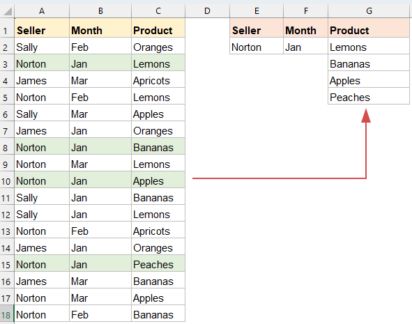
=TEXTJOIN(", ", TRUE, IF(($A$2:$A$18=E2)*($B$2:$B$18=F2), $C$2:$C$18, ""))
- ($A$2:$A$21=E2)*($B$2:$B$21=F2) تتحقّق مما إذا كان كل صف يستوفي الشرطين معًا: «البائع يساوي E2» و«الشهر يساوي F2». فإذا تحقّق الشرطان معًا، تكون النتيجة 1؛ وإلا فستكون 0. ويشير الرمز * إلى أن كلا الشرطين يجب أن يكونا صحيحَين.
- IF(..., $C$2:$C$21, «») تُرجع اسم المنتج إذا تطابق الصف، وإلا تُرجع خلية فارغة.
- TEXTJOIN(", ", TRUE, ...)تجمع جميع أسماء المنتجات غير الفارغة في خلية واحدة، مفصَّلة بـ "، ".
الطريقة 2: استخدام Kutools لـ Excel
يقدّم Kutools لـ Excel حلاً قويًّا وسهل الاستخدام يمكّنك من استرجاع القيم المطابقة المتعددة ودمجها في خلية واحدة بناءً على معايير متعددة—بدون الحاجة إلى صيغ معقّدة!
بعد تثبيت Kutools لـ Excel، يُرجى اتباع الخطوات التالية:
- حدد نطاق البيانات الذي ترغب في استخراج جميع القيم المقابلة له وفقًا للمعايير.
- ثم انقر فوق Kutools > دمج وتقسيم > دمج متقدم للصفوف، انظر لقطة الشاشة:

- في مربع حوار دمج متقدم للصفوف، يُرجى تهيئة الخيارات التالية:
- اختر رؤوس الأعمدة التي تحتوي على معايير المطابقة (مثل: البائع والشهر). ثم انقر فوق «المفتاح الأساسي» لكل عمود محدد لتعريفه كشرط بحث.
- انقر فوق رأس العمود الذي تريد استخراج نتائج الدمج منه (مثل: «المنتج»). ثم من قسم «الدمج»، اختر المُفصِّل المفضل لديك (مثل: فاصلة، مسافة، أو فاصل مخصص).
- وأخيرًا، انقر على زر «موافق».


النتيجة: سيقوم Kutools فورًا بدمج جميع القيم المطابقة في خلية واحدة لكل مجموعة معايير فريدة.
إرجاع قيم متعددة مطابقة بناءً على معايير متعددة في عمود
عندما تحتاج إلى استخراج وعرض سجلات مطابقة متعددة من مجموعة بيانات استنادًا إلى عدة شروط، وإرجاع النتائج بتنسيق عمودي، يوفّر Excel حلولًا قوية تلبي هذا الغرض.
الطريقة 1: استخدام صيغة مصفوفة (لجميع الإصدارات)
يمكنك استخدام صيغة المصفوفة التالية لإرجاع النتائج عموديًا في عمود:
1. انسخ أو أدخل الصيغة التالية في خلية فارغة:
=IFERROR(INDEX($C$2:$C$18, SMALL(IF(($A$2:$A$18=$E$2)*($B$2:$B$18=$F$2), ROW($C$2:$C$18)-ROW($C$2)+1), ROW(1:1))), "")2. اضغط على Ctrl + Shift + Enter للحصول على أول نتيجة مطابقة، ثم حدد الخلية الأولى التي تحتوي على الصيغة واسحب مقبض التعبئة لأسفل حتى تصل إلى خلية فارغة. الآن، تم إرجاع جميع القيم المطابقة كما في لقطة الشاشة التالية:

- $A$2:$A$18=$E$2: تتحقّق مما إذا كان البائع يطابق القيمة الموجودة في الخلية E2.
- $B$2:$B$18=$F$2: تتحقّق مما إذا كان الشهر يطابق القيمة في الخلية F2.
- * هو عامل منطقي AND (يجب أن يكون كلا الشرطين صحيحين).
- ROW($C$2:$C$18)-ROW($C$2)+1: يولّد رقم صف نسبي لكل منتج.
- SMALL(..., ROW(1:1)): تستخرج الصف الذي يحمل الرقم الأصغرn من بين الصفوف المطابقة (كلما سُحبت الصيغة لأسفل).
- INDEX(...): تُرجع القيمة من الصف المطابق.
- IFERROR(..., «»): تُرجع خلية فارغة إذا لم توجد مطابقات إضافية.
الطريقة 2: استخدام دالة FILTER (Excel 365 / 2021)
إذا كنت تستخدم Excel 365 أو Excel 2021، فإن دالة FILTER تُعد خيارًا ممتازًا لإرجاع نتائج متعددة استنادًا إلى معايير متعددة، بفضل بساطتها ووضوحها وقدرتها على عرض النتائج ديناميكيًّا دون الحاجة إلى صيغ مصفوفة معقدة.
انسخ الصيغة أدناه أو أدخلها في خلية فارغة، ثم اضغط مفتاح الإدخال (Enter)، وسيتم إرجاع جميع السجلات المطابقة استنادًا إلى المعايير المتعددة.
=FILTER(C2:C18, (A2:A18=E2)*(B2:B18=F2), "No match")
- FILTER(...) تُرجع جميع القيم من C2:C18 التي يتحقّق فيها الشرطان معًا.
- (A2:A18=E2)*(B2:B18=F2): مصفوفة منطقية تتحقّق من تطابق البائع والشهر.
- «No match»: رسالة اختيارية تُعرض إذا لم يتم العثور على أي قيم.
إرجاع قيم متعددة مطابقة بناءً على معايير متعددة في صف
غالبًا ما يحتاج مستخدمو Excel إلى استخراج قيم متعددة من مجموعة بيانات تحقق شروطًا محددة وعرضها أفقيًّا (ضمن صف واحد)—وهو أمرٌ مثالي لإنشاء تقارير ديناميكية، أو لوحات تحكم، أو جداول ملخّصة عندما تكون المساحة الرأسية محدودة. في هذا القسم، سنستعرض طريقتين فعّالتين لتحقيق ذلك.
الطريقة 1: استخدام صيغة مصفوفة (لجميع الإصدارات)
تسمح صيغ المصفوفة التقليدية باستخراج قيم مطابقة متعددة باستخدام دوال INDEX وSMALL وIF وCOLUMN. وعلى عكس الاستخراج الرأسي (المعتمد على الأعمدة)، يتم تعديل الصيغة لإرجاع النتائج في صف واحد.
1. انسخ الصيغة أدناه أو أدخلها في خلية فارغة:
=IFERROR(INDEX($C$2:$C$18, SMALL(IF(($A$2:$A$18=$E$2)*($B$2:$B$18=$F$2), ROW($C$2:$C$18)-ROW($C$2)+1), COLUMN(A1))), "")2. اضغط مفاتيح Ctrl + Shift + Enter للحصول على أول نتيجة مطابقة، ثم حدد الخلية التي تحتوي على الصيغة الأولى واسحب الصيغة إلى اليمين عبر الأعمدة لاسترداد جميع النتائج.

- $A$2:$A$18=$E$2: تحقّق مما إذا كان البائع متطابقًا.
- $B$2:$B$18=$F$2: تحقّق مما إذا كان الشهر متطابقًا.
- *: عامل AND المنطقي—يجب أن يكون الشرطان صحيحين معًا.
- ROW($C$2:$C$18)-ROW($C$2)+1: يُنشئ أرقام صفوف نسبية تُحدد عدد الصفوف.
- COLUMN(A1): يُحدِّد أي مطابقة سيتم إرجاعها، بناءً على المسافة التي تُسحَب بها الصيغة إلى اليمين.
- IFERROR(...): يمنع ظهور رسائل الخطأ بعد استنفاد جميع المطابقات.
الطريقة 2: استخدام دالة Filter (Excel 365 / 2021)
انسخ الصيغة أدناه أو أدخلها في خلية فارغة، ثم اضغط مفتاح الإدخال (Enter)، وسيتم استخراج جميع القيم المطابقة ووضعها في صف. انظر لقطة الشاشة:
=TRANSPOSE(FILTER(C2:C18, (A2:A18=E2)*(B2:B18=F2), "No match"))
- FILTER(...): تستخرج القيم المطابقة من العمود C وفقًا للشرطين.
- (A2:A18=E2)*(B2:B18=F2): يجب أن يتحقّق الشرطان معًا.
- TRANSPOSE(...): تحوّل المصفوفة العمودية التي تُرجعها دالة FILTER إلى مصفوفة أفقية.
🔚 الخاتمة
يمكنك استرجاع قيم مطابقة متعددة بناءً على معايير متعددة في Excel بعدة طرق، وذلك حسب الطريقة التي تفضلها لعرض النتائج—سواءً في عمود أو صف أو داخل خلية واحدة.
- يقدّم مستخدمو Excel 365 أو Excel 2021 دالة FILTER كحلٍ عصري، ديناميكي وأنيق يقلل التعقيد.
- أما بالنسبة لمستخدمي الإصدارات الأقدم، فلا تزال صيغ المصفوفة أدوات قوية، رغم أنها تتطلب إعدادًا وعناية أكثر قليلاً.
- بالإضافة إلى ذلك، إذا كنت ترغب في توحيد النتائج في خلية واحدة أو تفضّل حلاً لا يتطلب كتابة أكواد، فإن دالة TEXTJOIN أو أدوات الجهات الخارجية مثل Kutools لـ Excel يمكن أن تبسّط العملية بشكل كبير.
اختر الطريقة الأنسب لإصدار Excel الخاص بك والتخطيط الذي تفضّله، وستكون مجهّزًا جيدًا للتعامل مع عمليات البحث متعددة المعايير بكفاءة ودقة. إذا كنت مهتمًّا باستكشاف المزيد من نصائح وحيل Excel،فإن موقعنا يوفّر آلاف الدروس التعليمية لمساعدتك على إتقان Excel.
مقالات ذات صلة إضافية:
- إرجاع قيم نطاق قيمة البحث متعددة في خلية واحدة مفصولة بفواصل
- في Excel، تُستخدم دالة VLOOKUP عادةً لإرجاع أول قيمة مطابقة من جدول البيانات، لكن في بعض الأحيان نحتاج إلى استخراج **جميع** القيم المطابقة وعرضها في خلية واحدة مفصولة بمُفَصِّل معيّن—مثل فاصلة أو شرطة—كما في لقطة الشاشة التالية. كيف يمكننا استخراج جميع القيم المطابقة لقيمة البحث وإرجاعها في خلية واحدة مفصولة بفواصل في Excel؟
- بحث عمودي (VLOOKUP) وإرجاع قيم مطابقة متعددة دفعة واحدة في ورقة Google
- تُمكّنك دالة البحث العمودي (VLOOKUP) العادية في ورقة Google من العثور على أول قيمة مطابقة وإرجاعها بناءً على بيانات معيّنة. لكن في بعض الأحيان، قد تحتاج إلى إجراء بحث عمودي يُرجع **جميع** القيم المطابقة، كما في لقطة الشاشة التالية. هل لديك طريقة جيدة وسهلة لإنجاز هذه المهمة في ورقة Google؟
- بحث عمودي (VLOOKUP) وإرجاع قيم متعددة من قائمة منسدلة
- في Excel، كيف يمكنك تنفيذ بحث عمودي (VLOOKUP) لإرجاع جميع القيم المطابقة المرتبطة بعنصر معيّن من قائمة منسدلة دفعة واحدة—تمامًا كما يظهر في لقطة الشاشة التالية؟ في هذا المقال، سأرشدك إلى الحل خطوة بخطوة.
- بحث عمودي (VLOOKUP) وإرجاع قيم متعددة عموديًا في Excel
- عادةً، تُستخدم دالة VLOOKUP للحصول على أول قيمة مطابقة، لكن في بعض الأحيان قد تحتاج إلى إرجاع جميع السجلات المطابقة وفقًا لمعيار معيّن. في هذا المقال، سأشرح لك كيفية تنفيذ بحث عمودي (VLOOKUP) لإرجاع جميع القيم المطابقة—سواءً عموديًا، أفقيًا، أو حتى داخل خلية واحدة!
- بحث عمودي (VLOOKUP) وإرجاع البيانات المطابقة بين قيمتين في Excel
- في Excel، يمكننا استخدام دالة VLOOKUP العادية للحصول على القيمة المقابلة بناءً على بيانات معيّنة. ولكن في بعض الأحيان نريد تنفيذ بحث عمودي (VLOOKUP) وإرجاع القيمة المطابقة بين قيمتين كما في لقطة الشاشة التالية. كيف يمكنك التعامل مع هذه المهمة في Excel؟
أفضل أدوات الإنتاجية لمكتبتك
عزِّز مهاراتك في Excel باستخدام Kutools لـ Excel، وعايش الكفاءة كما لم تفعل من قبل.يقدّم Kutools لـ Excel أكثر من 300 ميزة متقدمة لتعزيز الإنتاجية ووقت الحفظ.انقر هنا للحصول على الميزة التي تحتاجها أكثر من غيرها...
يجلب Office Tab واجهة ذات علامات تبويب إلى Office، ويجعل عملك أسهل بكثير
- تمكّن من التحرير والقراءة باستخدام علامات التبويب في Word وExcel وPowerPoint، وPublisher وAccess وVisio وProject.
- افتح وأنشئ مستندات متعددة في علامات تبويب جديدة داخل النافذة نفسها، بدلاً من فتح نوافذ جديدة.
- يزيد إنتاجيتك بنسبة 50% ويوفّر لك مئات نقرات الفأرة كل يوم!
جميع الإضافات من Kutools في برنامج تثبيت واحد!
Kutools for Office حزمةٌ تحتوي على إضافاتٍ مخصصة لتطبيقات Excel وWord وOutlook وPowerPoint، إلى جانب Office Tab Pro، مما يجعلها الخيار المثالي للفِرق التي تعمل عبر تطبيقات Office.
- حزمة شاملة واحدة— إضافات Excel وWord وOutlook وPowerPoint بالإضافة إلى Office Tab Pro
- برنامج تثبيت واحد، ترخيص واحد— الإعداد خلال دقائق (جاهز لـ MSI)
- يعمل بشكل أفضل معًا— إنتاجية ميسَّرة عبر تطبيقات Office
- تجربة مجانية لمدة 30 يومًا بكامل الميزات— بدون تسجيل، بدون بطاقة ائتمان
- أفضل قيمة— وفِّر مقارنةً بشراء الإضافات بشكل منفصل