كيف يمكن تحويل الأرقام السالبة إلى موجبة في Excel؟
عند العمل في Excel، قد تحتاج أحيانًا إلى تحويل الأرقام السالبة إلى موجبة أو العكس. هل تبحث عن حيل سريعة لإنجاز ذلك؟ يقدم لك هذا المقال طرقًا فعّالة لتحويل جميع الأرقام السالبة إلى موجبة — أو العكس — بسهولة وسلاسة.
تغيير الأرقام السالبة إلى موجبة باستخدام دالة لصق خاص
تغيير الأرقام السالبة إلى موجبة بسهولة باستخدام Kutools لـ Excel
استخدام كود VBA لتحويل جميع الأرقام السالبة في نطاق ما إلى أرقام موجبة
تغيير الأرقام السالبة إلى موجبة باستخدام دالة لصق خاص
يمكنك تغيير الأرقام السالبة إلى أرقام موجبة باتباع الخطوات التالية:
1. أدخل الرقم-1 في خلية فارغة، ثم حدد هذه الخلية واضغط على مفاتيحCtrl + C لنسخه.
2. حدد جميع الأرقام السالبة في النطاق، ثم انقر بزر الماوس الأيمن واخترلصق خاص…من القائمة السياقية. راجع لقطة الشاشة: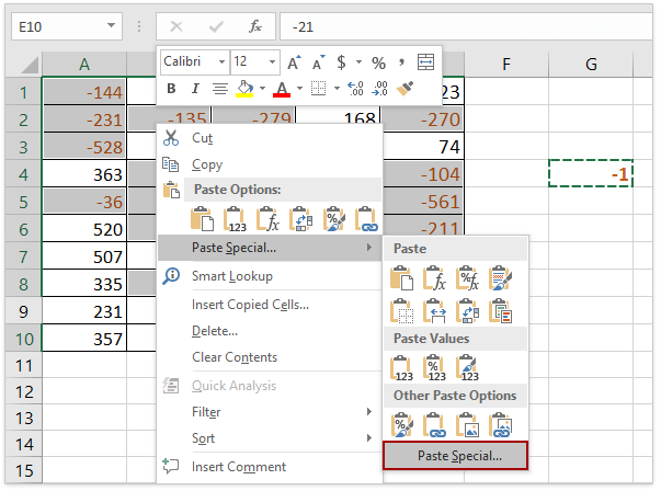
(1) عند الضغط باستمرار على مفتاحCtrl، يمكنك تحديد جميع الأرقام السالبة بالنقر عليها واحدة تلو الأخرى؛
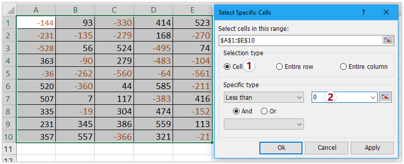
(2) إذا كان لديك Kutools لـ Excel مثبّتًا، فيمكنك استخدام ميزتهتحديد الخلايا الخاصةلتحديد جميع الأرقام السالبة بسرعة.جرّب النسخة المجانية!
3. ستظهر نافذة الحوارلصق خاص. اختر الخيارالكلمن قسماللصق، ثم اختر الخيارضربمن قسمالعملية، وأخيرًا انقر علىموافق. راجع لقطة الشاشة:
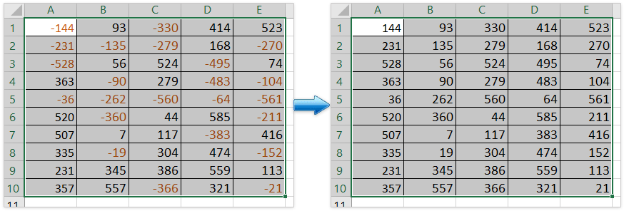
4. سيتم تحويل جميع الأرقام السالبة المحددة تلقائيًا إلى أرقام موجبة. احذف الرقم -1 عند الحاجة. راجع لقطة الشاشة:
تغيير الأرقام السالبة إلى موجبة بسرعة وسهولة باستخدام Kutools لـ Excel
معظم مستخدمي Excel لا يرغبون في استخدام كود VBA، فهل تبحث عن حيل سريعة لتغيير الأرقام السالبة إلى موجبة؟Kutools لـ Excelيمكنه مساعدتك على تحقيق ذلك بسهولة ويسر!
1. اختر نطاقًا يحتوي على الأرقام السالبة التي تريد تغييرها، ثم انقرKutools > المحتوى > تغيير علامة الرقم.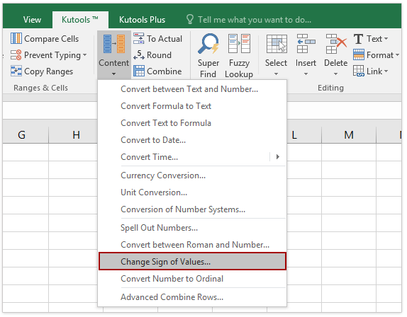
2. حدد خانةتغيير جميع الأرقام السالبة إلى موجبةضمن قسمالعملية، ثم انقرموافق. انظر لقطة الشاشة: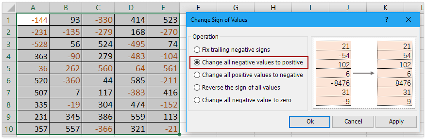
الآن سترى أن جميع الأرقام السالبة قد تحوّلت إلى أرقام موجبة كما هو موضح أدناه: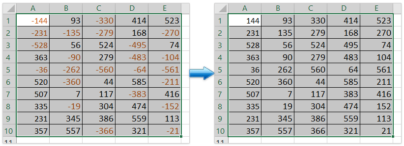
ملاحظة: باستخدام هذه الميزةتغيير علامة الرقم، يمكنك أيضًا تصحيح جميع الأرقام السالبة في النهاية، وتحويل جميع الأرقام الموجبة إلى سالبة، وعكس جميع الأرقام الموجبة والسالبة وتغيير جميع الأرقام السالبة إلى صفر.جرّبها مجانًا!
(1) تغيير جميع الأرقام الموجبة إلى سالبة بسرعة في نطاق محدود: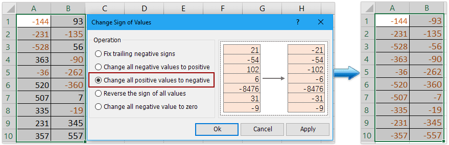
(2) عكس جميع الأرقام الموجبة والسالبة بسهولة في نطاق محدود: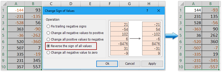
(3) تغيير جميع الأرقام السالبة إلى صفر بسهولة في نطاق محدود:
(4) تصحيح جميع الأرقام السالبة في النهاية بسهولة في نطاق محدود: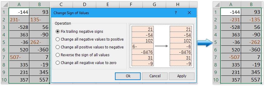
استخدام كود VBA لتحويل جميع الأرقام السالبة في نطاق ما إلى أرقام موجبة
بصفتك محترف Excel، يمكنك أيضًا تشغيل كود VBA لتحويل الأرقام السالبة إلى أرقام موجبة.
1. اضغط على مفتاحَي Alt + F11 لفتح نافذة Microsoft Visual Basic for Applications.
2. ستظهر نافذة جديدة. انقر فوقإدراج > وحدة نمطية (Module)، ثم أدخل الأكواد التالية في الوحدة النمطية:
Sub Positive
Dim Cel As Range
For Each Cel In Selection
If IsNumeric(Cel.Value) Then
Cel.Value = Abs(Cel.Value)
End If
Next Cel
End Sub3. بعد ذلك، انقر على زرتشغيلأو اضغط مفتاحF5 لتشغيل التطبيق، وسيتم تحويل جميع الأرقام السالبة إلى أرقام موجبة. انظر لقطة الشاشة:
مقالات ذات صلة
عكس إشارات القيم في الخلايا
عند استخدام Excel، تحتوي ورقة العمل عادةً على أرقام موجبة وسالبة. فماذا لو احتجنا إلى تحويل الأرقام الموجبة إلى سالبة، والعكس بالعكس؟ بالطبع، يمكننا تعديلها يدويًّا، لكن إذا كانت هناك مئات الأرقام التي تحتاج إلى تغيير، فهذه الطريقة ليست فعّالة على الإطلاق! هل تعلم أن هناك حيلًا ذكية وسريعة لحل هذه المشكلة؟
تحويل الأرقام الموجبة إلى سالبة
كيف يمكنك تحويل جميع الأرقام أو القيم الموجبة إلى سالبة بسرعة في Excel؟ تُظهر لك الطرق التالية كيفية تحويل جميع الأرقام الموجبة إلى سالبة في Excel بسهولة وسرعة.
تصحيح جميع الأرقام السالبة التي تظهر إشارتها في نهاية الخلايا
لسببٍ ما، قد تحتاج إلى تصحيح الأرقام السالبة التي تظهر علامتها في نهاية الخلايا في Excel. على سبيل المثال، قد يُعرض الرقم الذي يحتوي على علامة سالبة في نهايته بالشكل التالي: 90-. فكيف يمكنك إصلاح هذه العلامات السالبة بسرعة، ونقلها من نهاية الرقم إلى بدايته؟ إليك بعض الحيل السريعة التي ستساعدك على فعل ذلك!
تغيير الأرقام السالبة إلى صفر
سأريك كيف تحوّل جميع الأرقام السالبة إلى أصفار دفعة واحدة داخل النطاق المحدد!
أفضل أدوات الإنتاجية للمكتب
Kutools لـ Excel - يساعدك على التميّز بين الحشود
Kutools لـ Excel يضم أكثر من 300 ميزة،مما يضمن أن ما تحتاجه يكون على بعد نقرة واحدة فقط...
Office Tab - تمكين القراءة والتحرير باستخدام علامات التبويب في Microsoft Office (بما في ذلك Excel)
- ثانية واحدة للتبديل بين عشرات المستندات المفتوحة!
- يوفر لك مئات النقرات كل يوم، وقل وداعًا لآلام اليد الناتجة عن استخدام الفأرة!
- يزيد إنتاجيتك بنسبة 50% عند عرض وتحرير عدة مستندات في آنٍ واحد.
- يُدخل Tabs ميزة التبويبات الفعّالة إلى Office (بما في ذلك Excel)، تمامًا كما في Chrome وEdge وFirefox.