كيف يمكن استخدام دالة VLOOKUP لإرجاع أعمدة متعددة من جدول في Excel؟

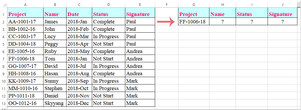
في ورقة عمل Excel، يمكنك استخدام دالة VLOOKUP لإرجاع القيمة المطابقة من عمود واحد. لكن في بعض الأحيان، قد تحتاج إلى استخراج القيم المطابقة من أعمدة متعددة، كما يظهر في لقطة الشاشة التالية. فكيف يمكنك الحصول على القيم المقابلة دفعة واحدة من أعمدة متعددة باستخدام دالة VLOOKUP؟

استخدام VLOOKUP لجلب القيم المطابقة من أعمدة متعددة بواسطة صيغة صفيف

استخدام VLOOKUP لجلب القيم المطابقة من أعمدة متعددة بواسطة صيغة صفيف

هنا، سأقدّم لك كيفية استخدام دالة VLOOKUP لإرجاع القيم المطابقة من أعمدة متعددة، يُرجى اتباع الخطوات التالية:

1. حدد الخلايا التي ترغب في ملئها بالقيم المطابقة من الأعمدة المتعددة، كما هو موضح في لقطة الشاشة التالية:

2. بعد ذلك، أدخل الصيغة التالية في شريط الصيغة، ثم اضغط على مفاتيح Ctrl + Shift + Enter معًا—وستُستخرج القيم المطابقة من الأعمدة المتعددة دفعةً واحدة! راجع لقطة الشاشة:

=VLOOKUP(G2,A1:E13,{2,4,5},FALSE)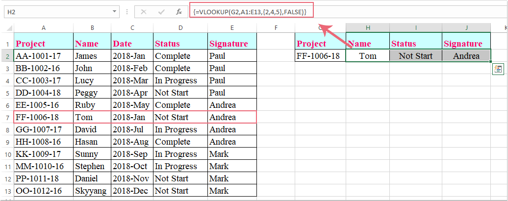

ملاحظة: في الصيغة أعلاه، يُمثل G2 المعيار الذي تريد استرجاع القيمة بناءً عليه، ويشير A1:E13 إلى نطاق الجدول الذي يتم تنفيذ دالة VLOOKUP منه، بينما تشير الأرقام 2 و4 و5 إلى أرقام الأعمدة التي تريد استرجاع القيم منها.

تغلّب على حدود VLOOKUP مع Kutools: بحث متقدم

للتغلب على القيود المفروضة على دالة VLOOKUP في Excel، طوّرت Kutools مجموعةً من ميزات البحث المتقدمة التي توفر للمستخدمين حلاً أكثر قوةً ومرونةً للعثور على بياناتهم.

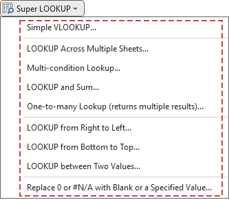
• 🔍بحث في عدة ورقات...: ابحث عبر أوراق عمل متعددة للعثور على البيانات المطابقة بسهولة وسرعة.
• 📝البحث - البحث بشروط متعددة...: ابحث عن البيانات التي تحقّق عدة معايير في آنٍ واحد.
• ➕البحث والتجميع...البحث والمجموع...: ابحث عن البيانات بناءً على قيمة معيّنة، ثم اجمع النتائج.
• 📋)بحث واحد إلى العديد (إرجاع نتائج متعددة...): استرجع قيمًا مطابقة متعددة لمُدخل بحث واحد.
• احصل على Kutools لـ Excel الآن!

أفضل أدوات الإنتاجية لمكتبتك

🤖	KUTOOLS AI مساعد: ثوّر تحليل البيانات استنادًا إلى:التنفيذ الذكي   |  إنشاء الكود|  إنشاء الصيغ المخصصة  |  تحليل البيانات وإنشاء المخططات البيانية|  استدعاء الوظائف المحسنة…
	الميزات الشائعة:البحث، التمييز أو وضع علامة على المكررات   |  حذف الصفوف الفارغة   |  دمج الأعمدة أو الخلايا دون فقدان البيانات   |  التقريب بدون استخدام الصيغة...
	بحث متقدم:VLookup متعدد المعايير  |  VLookup متعدد القيم  |   VLookup عبر أوراق متعددة   |   مطابقة غامضة....
	قائمة منسدلة متقدمة:إنشاء قائمة منسدلة بسرعة   |  قائمة منسدلة تابعة   |  قائمة منسدلة متعددة الاختيار....
	مدير الأعمدة:إضافة عدد محدد من الأعمدة|نقل الأعمدة|تبديل حالة ظهور الأعمدة المخفية|مقارنة النطاقات والأعمدة...
	ميزات مميزة:التركيز على الشبكة   |  عرض التصميم   |شريط الصيغ المحسن   | مدير الدفتر والورقة   |  مكتبة الموارد(نص تلقائي)|  أداة اختيار التاريخ   |  تجميع ورقات العمل  |  تشفير/فك تشفير الخلايا   | إرسال رسائل البريد الإلكتروني حسب القائمة   |  مرشح متقدم   |   تصفية خاصة(تصفية الخلايا التي تحتوي على خط عريض/مائل/يتوسطه خط...) ...
	أفضل 15 مجموعات الأدوات:12 أدواتالنصوص(إضافة نص،حذف الأحرف المحددة، ...)|   50+أنواعالمخططات البيانية(مخطط جانت، ...)|   40+ صيغعملية(حساب العمر بناءً على تاريخ الميلاد، ...)|   19 أدواتالإدراج(إدراج رمز QR،إدراج صورة من المسار، ...)|   12 أدواتالتحويل(تحويل إلى كلمات،تحويل العملة، ...)|   7 أدواتدمج وتقسيم(دمج متقدم للصفوف،تقسيم الخلايا، ...)|... وأكثر من ذلك

استخدم Kutools باللغة التي تفضلها – يدعم الإنجليزية والإسبانية والألمانية والفرنسية والصينية و40+ لغات أخرى!

عزِّز مهاراتك في Excel باستخدام Kutools لـ Excel، وعايش الكفاءة كما لم تفعل من قبل.يقدّم Kutools لـ Excel أكثر من 300 ميزة متقدمة لتعزيز الإنتاجية ووقت الحفظ.انقر هنا للحصول على الميزة التي تحتاجها أكثر من غيرها...

مزيد من التفاصيل حول Kutools لـ Excel...تنزيل مجاني...

---

يجلب Office Tab واجهة ذات علامات تبويب إلى Office، ويجعل عملك أسهل بكثير

• تمكّن من التحرير والقراءة باستخدام علامات التبويب في Word وExcel وPowerPoint، وPublisher وAccess وVisio وProject.
• افتح وأنشئ مستندات متعددة في علامات تبويب جديدة داخل النافذة نفسها، بدلاً من فتح نوافذ جديدة.
• يزيد إنتاجيتك بنسبة 50% ويوفّر لك مئات نقرات الفأرة كل يوم!

مزيد من التفاصيل حول Office Tab...تنزيل مجاني...

---

جميع الإضافات من Kutools في برنامج تثبيت واحد!

Kutools for Office حزمةٌ تحتوي على إضافاتٍ مخصصة لتطبيقات Excel وWord وOutlook وPowerPoint، إلى جانب Office Tab Pro، مما يجعلها الخيار المثالي للفِرق التي تعمل عبر تطبيقات Office.

• حزمة شاملة واحدة— إضافات Excel وWord وOutlook وPowerPoint بالإضافة إلى Office Tab Pro
• برنامج تثبيت واحد، ترخيص واحد— الإعداد خلال دقائق (جاهز لـ MSI)
• يعمل بشكل أفضل معًا— إنتاجية ميسَّرة عبر تطبيقات Office
• تجربة مجانية لمدة 30 يومًا بكامل الميزات— بدون تسجيل، بدون بطاقة ائتمان
• أفضل قيمة— وفِّر مقارنةً بشراء الإضافات بشكل منفصل

مزيد من التفاصيل حول Kutools for Office...تنزيل مجاني...